This article presents an Audio Content Identification method inspired to a popular recognition model from the Computer Vision community, namely the “visual words” model, which is a powerful framework for the representation of images based on concepts from the Information Retrieval field used for text-based search. The method utilizes efficient local binary descriptors combined with machine learning techniques to build an audio fingerprinting model for the representation of sound based on “auditory words”. This model forms the basis of an audio recognition system powered by a flexible multi-level matching algorithm.
1. Introduction
In a world that is becoming increasingly interconnected and where social media are used by more and more people the production of multimedia content is exponentially growing and with this comes the need for tools to analyze huge amounts of data in order to extract useful information. Also, the rapid adoption of automation in basically all aspects of our life will probably give rise to new services and products that will benefit from Audio Content Identification (ACI) technology (for example in robotics and machine listening). All this has drawn the attention of the research community in recent years for the development of efficient methods to perform automatic processing of audio/visual data in order to recognize high level contents.
While the human vision system has been extensively studied revealing much of the inner workings at both the sensorial level (the eye) and cognitive level (visual cortex) allowing the computer vision field to make substantial progress, it seems the auditory system in the Artificial Intelligence world has not received as much attention and the amount of research devolved to the artificial vision field still appears to be by far superior. This is probably due to the fact that we’re mostly vision-driven creatures and there are perhaps more applications for computer vision systems than for ACI systems. Despite this, in the audio identification realm there are many approaches that can be directly mapped to methods used in computer vision and it is not unusual, therefore, to see computer vision techniques transferred to the audio recognition field in order to solve similar problems. In this article we show how techniques borrowed from disciplines outside audio processing can be used with success to design a high performance audio content recognition system.
2. Audio fingerprinting using audio components
The concept of fingerprint has been extensively used in several fields as a mean to identify entities from their unique features and audio fingerprinting is the technique that uses this concept for audio content identification. The main idea is that of extracting perceptually meaningful features that best characterize the audio signals in order to build a compact “signature” that can later be used to identify specific content from unknown audio data. Many methods have been developed in recent years that use different fingerprint models, from physiologically motivated approaches based on a model of the inner ear that decomposes the audio signal into its frequency components using the DFT and some kind of filterbank from which to extract relevant features, such as in [1], to methods using statistical classifiers to discover perceptually meaningful audio components [2], landmark points over 2D representations of sound [3], combinatorial hashing [4] and clustering [5].
Some interesting methods have been proposed that use computer vision techniques, notably the works of [6] and [7] have shown the validity of this approach. The motivation behind this idea is that most audio fingerprinting methods use some sort of 2D representation of the audio signal (Spectrogram, Chromagram, Cochleogram, etc.) and such representations can be directly used to extract features using 2D computer vision techniques in order to build robust and efficient fingerprints. In the following sections we show how, following this approach, not only it is possible to use computer vision processing techniques (such as descriptors extraction) but also to adopt entire models and paradigms to solve audio identification problems.
2.1 Audio components
Many approaches used in computer vision are physiologically motivated by the human vision system, which uses low level components such as corners, lines and textures to represent objects, and that are all based on intensity variations, the primary feature used by the human brain to recognize objects. So, for example, a set of lines and corners with a specific spatial relationship may represent an eye, mouth, or ear, which, in turn, may be part of a more complex object (a face).
An image recognition model based on these concepts has been proposed in the computer vision community [14] and has proven successful in the identification of visual objects. This model, called the “visual words” model, is based on the idea of decomposing a complex entity into smaller components, that can easily be represented in a symbolic way, and represent the entity as a connected structure of these components, the same way a sentence is represented by syntactically connected words.
Following this approach, we can think that the auditory system uses low level components as well as a primary representation of sounds. These audio components are characterized by their time-frequency distribution of intensity, the same as low level visual features are characterized by their intensity distribution on the 2D space. Examples of audio components used to recognize sounds are:
Noise-like components
The main feature of these components is the absence of a structured pattern and the random distribution of energy across a broad frequency band. Examples of sounds where they can be found include utterance (some consonants), percussion instruments and many ambient sounds.
Tone-like components
These are audio components characterized by energy distributions across a frequency range following a periodic pattern. This periodic-like pattern along frequency is due to the harmonic content of the sound, which vary depending on its nature. Another characteristic of these components is their fundamental frequency, which is used to determine the “pitch” of the sound. Typical sounds where they can be found include utterance (vowels) and the sound of most music instruments.
Pulse-like components
Audio components characterized by uniform intensity distribution across a broad frequency range with high impulsiveness (high energy released in a very short period of time, usually tens of milliseconds). Typical examples of such components can be found in many percussion instruments, utterances (consonants) and other “beat-like” sounds.

Any sound can be seen as a combination of these type of audio components to form a time-space structure representing an auditory scene. This concept is used in some audio recognition systems, for example in the method proposed by Cano et al. [2] who used a model based on audio components called “audio genes” learned from music data sets using HMMs.
Using these ideas, we propose an approach that aims at building a suitable representation of sound based on the above mentioned audio components, which we call auditory words, in order to design a robust audio fingerprinting scheme for audio content identification. In the following section a detailed explanation of the method is given.
2.2 Audio Descriptors
The preprocessing stage in audio fingerprinting usually involves the transformation of the signal from the original time domain into a more suitable space. Many methods work using a psychoacoustically motivated frequency domain obtained by applying some form of sub-band decomposition to the DFT, such as the Mel Scale, Bark Scale, etc. This is mainly due by the need of reducing the computational burden, and also an attempt to mimic the way the inner ear process sounds. In our method we do not use such approach as the aggregation process in the construction of these sound representations will suppress important information that need to be captured by the descriptors used in the model, and also, the nature of these descriptors and the way they are localized already perform a sort of “compression” on the original spectral signal reducing the computational cost. This will be clearer in the following sections.
Most of the useful information carried by audio signals to human listeners lie in the frequency range 100-3000 Hz, so the original signal is resampled to 11025 Hz and transposed to the frequency domain by applying the Short Time Fourier Transform (STFT) with a window size of 1024 samples and a hop time of 13.88 ms smoothed using the Hamming window.
A key issue is the representation of the auditory words in a manner that the resulting fingerprints are compact, with a good discriminative power and able to recognize audio from very short clips extracted at any point within a recording, in order to be suitable for real-time applications. Specifically we want descriptors that are
1. Locally informative
2. Stable
3. Compact and fast to compare
4. Time-translation invariant
Point 1 means that the descriptors must carry enough information so to be highly discriminative and must capture local features within the audio. They must also be highly reproducible, that is, the points at which they’re computed (Points Of Interest) must be stable in order to survive noise and other signal transformations. Given the amount of data produced nowadays, we also want them to be compact in order to yield fingerprints with low storage requirements and that can be compared quickly using fast similarity metrics. In the following section we describe how we find good locations in the time-frequency space in order to extract the audio descriptors.
2.3 Points Of Interest
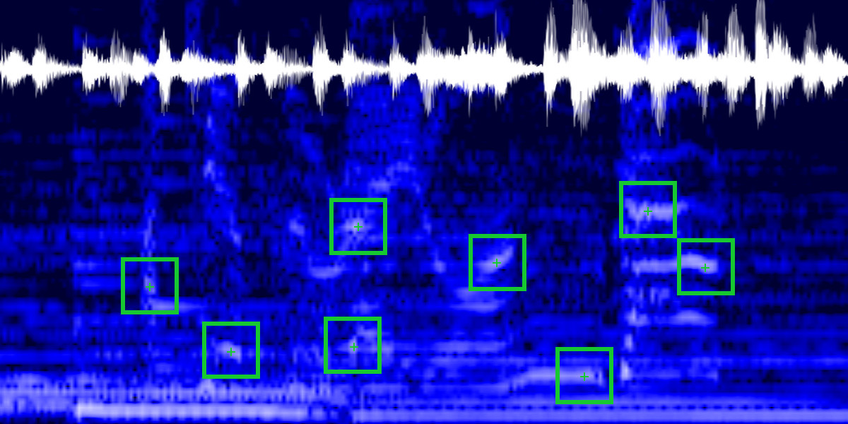
 Audio events usually do occur at locations where there are consistent energy variations in time and frequency. The works in [3] and [4] have shown that spectral peaks alone are good descriptors yielding high recognition accuracy. We also second this choice with the motivation that peaks usually occur at locations where there are onsets, which have been extensively used in audio processing as a feature. The definition of onset vary in the literature depending on the application, but a common one is to define them as sudden bursts of energy with the envelope shown in Figure 2. Onsets are related to various audio sources, (instrument notes, vocals, natural processes, etc.) and the transient part is usually associated with peaks in the frequency domain, thus to locate points of interest we look for “consistent peaks” in the STFT spectrum. A consistent peak is defined as a small, well localized burst of energy defined by its maximum M, width W, as shown in Figure 3

and energy content \(E_{P}\) defined as follows
\(E_{P}=\displaystyle\sum_{p \in W \times W} |STFT(p)|^{2} \tag{1}\)
The detection of the POIs is done in 2 stages: in the first stage we scan the STFT spectrum for candidate points. This is accomplished by convolving the spectrum with the following Laplacian parametric kernel
\(H = \begin{bmatrix} -1 & -1 & -1 \\ -1 & k & -1 \\ -1 & -1 & -1 \end{bmatrix} \tag{2}\)
which approximates the second order derivative of the signal. Looking at the positive response of the filter we search for local maxima in order to detect good candidates. The k parameter is a boosting factor that determines the sensitivity of the filter to the peaks and should be properly set to avoid the selection of local maxima that are not consistent enough (weak peaks). In our experiments we noticed the best values to be in the range [6,7]. The result of this stage is the set of candidates
\(C_{1} = \{ p | STFT(p) \ast H > 0 \} \tag{3}\)
However, the filtering in stage 1 will also be picking many inconsistent POIs, so the second stage aims at rejecting these points by performing a non-maximum suppression filtering on \(C_{1}\). Each candidate in \(C_{1}\) is processed by centering a window \(W{p}\) in p and taking the peak with maximum energy in it. The final set of detected POIs is then obtained as follows
\(C_{POI}=\{p \in C_{1} | p=\underset{p \in W_{p}}{\arg\max} ~ E_{P}(p) \} \tag{4}\)
The size of the non-maximum suppression window \(W_{p}\) determines the sparsity of the detected POIs and, therefore, the granularity of the fingerprints. In our implementation we use a window size of 400 ms \(\times\) 340 Hz.
2.4 Local Binary Descriptors
There is an interesting class of descriptors that fulfill all of the requirements stated in 2.2, called Local Binary Descriptors, becoming increasingly popular in the computer vision field, and that have been proven to yield comparable accuracy to their continuous real-valued counterpart, while being easier to compute, more efficient to store and, most of all, way faster to compare.
Almost all of them are derived from or inspired to the Census Transform, introduced in [8], which is a form of non-parametric statistical method based on comparisons between data points rather than on the values of data points themselves. Descriptors based on this approach can be found in [9][10][11] and have been shown to outperform those based on standard parametric statistics in many aspects, especially when it comes to speed of computation, comparison and storage requirements.
Formally, given a data point p and a neighborhood \(N(p)\), the census transform maps \(N(p)\) to a bit string d, as follows
\(d(p) = \displaystyle\bigcup_{p’ \in N(p)} b(p,p’) \tag{5} \)
where \(b(p,p’)\) is some comparison binary function. Our binary descriptor is also derived from this method and is computed in a “shift & overlap” fashion as follows:
At each POI \(p \in C_{POI}\) a neighborhood \(N(p)\) of extension \(\Delta F_{N(p)} \times \Delta T_{N(p)}\) is considered. The size of \(N(p)\) should be chosen so that enough dynamics is captured for the resulting auditory words to have good discriminative power. There is a trade-off between performance and accuracy to keep into account as too big neighborhoods will capture more information but will increase the size of the descriptors affecting performances, while too small sizes may yield descriptors with poor informative content affecting accuracy. We empirically found a satisfactory value to be around 300 ms \(\times\) 200 Hz.
\(N(p)\) is then scanned sliding a small window \(W_{c}\) of size \(\Delta F_{W(c)} \times \Delta T_{W(c)}\) with a stride of \(s=(s_{t},s_{f})\) at evenly spaced points p’, as depicted in Figure 4(a). The overlapping between sliding windows helps with capturing more detailed information about the dynamics of the audio and makes the descriptors more robust to inaccuracies in the detection of the POIs.
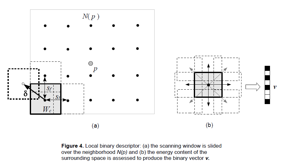
For each scanning window \(W_{c}\) at each scanning point p’ the Mean Energy \(E^{\mu}_{Wc}\) is computed and compared to those of its k-neighborhood, given by moving \(W_{c}\) in the k directions, as depicted in Figure 4(b). The Mean Energy gradients are then mapped to the binary space using the following function
\(b(p’,p’+\delta) = \begin{cases} 1 & \text{if } E^{\mu}_{Wc}(p’)-E^{\mu}_{Wc}(p’+\delta)>0 \\ 0 & \text{otherwise} \end{cases} \tag{6}\)
where \(E^{\mu}_{Wc}\) is given by
\(\displaystyle E^{\mu}_{Wc} = \frac{1} {|W_{c}|} \sum_{p \in W_{c}} |STFT(p)|^{2} \tag{7}\)
and δ is the displacement in the k directions. This process yelds a binary vector \(\textbf{v} \in \{0,1\}^{k} \) for each scanning window in \(N(p)\) whose components are given by (6). This “sub-descriptor” captures the spatio-temporal relations between local audio events and their concatenation produces the final binary descriptor \(d(p)\) for \(N(p)\) given by
\(d(p) = \displaystyle\bigoplus_{W_{c} \in N(p)} \textbf{v}(W_{c}) \tag{8}\)
The process of assembling the final binary descriptor is depicted in Figure 4(c). Note that the scanning directions are not relevant. In the picture it is horizontal but it may as well be vertical.

The number of scanning windows \(W_{c}\) and the neighborhood k will determine the size of the descriptor. Specifically, if \(N_{W_{c}}\) is the number of scanning windows, then the size of \(d(p)\) will be
\(|d(p)| = k \cdot N_{W_{c}} \tag{9}\)
where \(N_{W_{c}}\), in turn, depends on the strides used to scan \(N(p)\). In our experiments we used a 4-neighborhood (k=4) in the N-E-S-W directions and a stride/displacement of 50%. Using a 4-neighborhood rather than a fully connected 8-neighborhood we didn’t notice any significant reduction in the recognition accuracy, while reducing the size of the descriptors (and thus of the fingerprints database) by a factor of 2. The size of \(W_{c}\) was set to 50ms \(\times\) 35Hz.
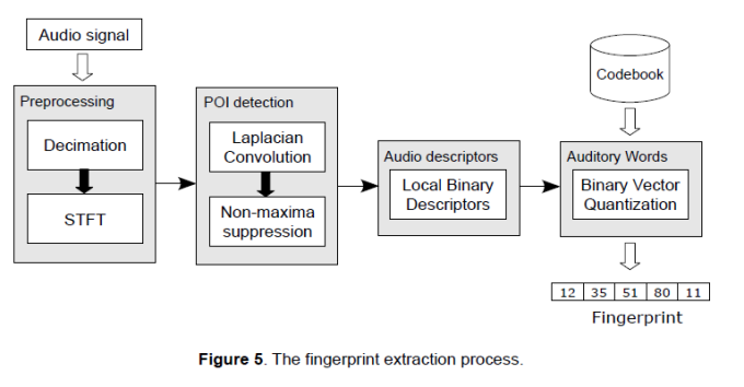
The process described so far represents the fingerprints extraction stage and it’s depicted in Figure 5. The input to this stage is the original audio signal while the output is the fingerprint, which is an ordered sequence of auditory words each one representing a sub-fingerprint, here called Local Fingerprints (LF), along with some supporting information. Each LF is a n-tuple \(s=\langle d,t,f \rangle\), which will be transformed into \(s=\langle w,e,t,f \rangle\) by the quantization stage. The global fingerprint of the audio is then represented by this ordered sequence of Local Fingerprints \(F=\{s_{j}\}, ~ j=1,2,…,n\) .
2.5 Binary Vector Quantization
Vector Quantization is a popular machine learning technique used to discover patterns in large data sets and to reduce the feature space in order to improve the efficiency of the algorithms. In our case each descriptor is a vector representing the local spatio-temporal evolution of the audio signal that is perceptually modeled as audio components, which collectively produce a certain sound. Specifically, they are, with the current settings, 720-bit vectors in the binary vector space. It is reasonable to think that small variations in these spatio-temporal evolutions are still perceived as the same sound, hence it makes sense to cluster this vector space in order to learn a set of representative vectors into which to map the whole descriptor space. This set of vectors (the codebook) forms the auditory words, which should be able to capture as much as possible the statistics of the data set in order to describe it with good accuracy. This is usually accomplished by running some clustering algorithms on the data set, among which k-means is a very popular one. This approach has been used in the computer vision field for image recognition.
However, in our case descriptors are represented by binary vectors and we want to find native methods in order to operate within the binary vector space. Although k-means has been also used for binary vector quantization ([12]), it would defeat our requirements of compactness and fast similarity computation as it would require working in the real domain using real-valued metric distances. In our method we perform binary vector quantization using k-medians instead, which is based on the evaluation of representative binary vectors using a quick procedure and the Hamming distance for similarity computation, which is faster than the real-valued Euclidean distances. The algorithm proceeds as follows:
1. From a data set \(D \subset [0,1]^{n}\) of binary descriptors extract a subset \(V \subset D\). This subset (also called the “training set”) should be highly heterogeneous in the chosen domain in order to capture as much as possible of the underlying statistics describing D. For example, for music it should contain songs of many different genres.
2. Perform k-means++ seeding to pick the initial centroids \(C(t_{0})=\{c_{1},…,c_{k}\}\) from V, as follows:
2.1 – Sample a point \(v \in V\) at random from a uniform distribution as the initial centroid \(c_{1}(t_{0})\).
2.2 – For each remaining centroid \(c_{j}(t_{0}), ~ j=2…k\):
2.2.1 – Compute the p.d.f. of the points \(v \in V\) according to the following
\(p(v) = \frac{\displaystyle\min_{c_{j} \in C} \|v-c_{j}\|} {\displaystyle\sum_{k=1}^{|V|} min_{c_{j} \in C} \|v_{h}-c_{j}\|} \tag{10}\)
where \(\|\bullet\|\) denotes Hamming distance.
2.2.2 – Sample a point \(v \in V\) at random from the non-uniform distribution given by p(v) using Inverse Transform Sampling, as follows:
I) Generate a probability value \(u \in [0,1]\) at random from a uniform distribution.
II) Take the point \(\bar{v}\) such that \(F(\bar{v})>u\) where
\(F(\bar{v})=\displaystyle\sum_{v=1}^{\bar{v}} p(v) \tag{11}\)
is the cumulative distribution function.
III) Set \(c_{j}=\bar{v}\) and add it to \(C(t_{0})\).
3. Perform k-medians according to the following algorithm:
3.1 – Form \(S_{j}(t)=\{v \in V | argmin_{c \in C(t)} \|v-c_{j}\| \}\) clusters by grouping all \(v \in V\) that are closer to centroid \(c_{j}\) than any other v.
3.2 – Compute new centroids \(C(t+1)\) by computing a median vector in each cluster \(S_{j}(t)\) as follows:
\(c_{j}(t+1)=[M(v_{1}),…,M(v_{n})]~~~~~\forall v \in S_{j}(t) \tag{12}\)
where \(M(v_{x})\) is given by the following function
\(M(v_{x}) = \begin{cases} 0 & \text{if } |Z_{x}|>|O_{x}| \\ 1 & \text{if } |Z_{x}|<|O_{x}| \\ c_{jx} & \text{if } |Z_{x}|=|O_{x}| \\ \end{cases} \tag{13}\)
and \(Z_{x}, O_{x}\), indicate the sets of zeroes and ones respectively for component x across all vectors in cluster \(S_{j}(t)\). Equation (13) effectively computes the median of a component and since vectors are binary this reduces to a simple count of how many ones and zeroes are in such component.
3.3 – Repeat until all clusters are stable. The stability can be assessed by checking that the vast majority of vectors are assigned to the same clusters between iterations or that some error function falls below a threshold.
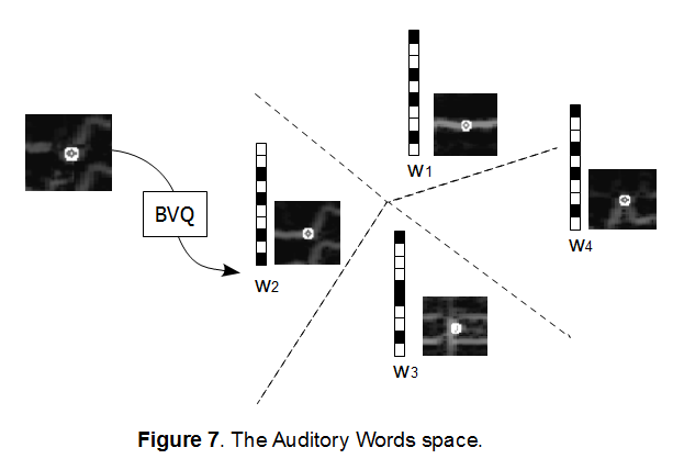
The resulting codebook will be the set of auditory words used for recognition. Examples of some auditory words learned by the algorithm are shown in Figure 7. We expect the dimension of this reduced feature space be much smaller than the dimension of the vector space in which the original descriptors live (a 720-dimensional space in our implementation), so that these words can be represented by a machine word (i.e. 8-64 bits).
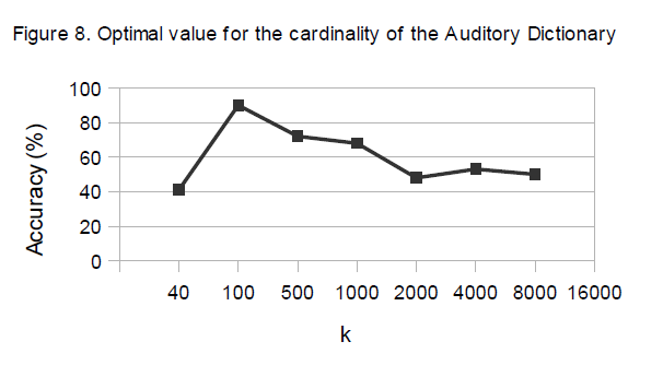
A key issue in the construction of a dictionary with k-medians is to find the optimal value for k. If it is too small, the dictionary may not be discriminative enough leading to a high rate of false positives. On the other hand, too many words could generate a dictionary that is too selective with a poor generalization power, leading to low robustness to noise.
From our experiments we noticed that the cardinality of this dictionary is very low. Probably the underlying language induced by the descriptors that we have built is quite limited and few patterns can already describe the whole data set with good accuracy, as can be seen in Figure 8. The graph shows that 100 words is the optimal number of auditory words, which means the original 720-dimensional feature space can be mapped into a reduced 7-dimensional binary vector space. The auditory words were learned from a music data set of 200 mixed genres songs and tested on another music data set using 200 query audio clips played over the air.
3. Matching
The fingerprinting method described in the previous sections yields compact fingerprints that are efficient in terms of storage requirement and similarity computation. While a full search of the fingerprint space by cross-correlation between the query and the references in a database to find the best match is feasible for small data sets, in real-world scenarios these data sets are usually large containing thousands or millions of documents, therefore a fast matching algorithm that quickly scans the fingerprint space to find the most similar objects to a query is paramount. Due to the way a fingerprint is represented, this process can be seen as the search for the most relevant document containing the given key words. Since the algorithm is designed for real-time audio streams processing, this is inherently an integrative process where incoming auditory words are processed in batches and evidence accumulated over time until there is a clear match. Formally, be \(R(\bullet,\bullet)\) a scoring function taking 2 arguments, X the unknown query sequence and F a reference fingerprint, then
\(R(X,F)=\displaystyle\sum_{n=1}^{N_{T}}R(X_{t}^{k},F) \tag{14}\)
is the cumulative score over \(N_{t}\) time steps, where \(X_{t}^{k}=\{w_{1},…,w_{k}\} \subset X\) indicates the set of auditory words at step t being processed. The matching problem can then be defined as
\(F_{match}=\underset{F \in D}{\arg\max}~R(X,F) \tag{15}\)
In the following sections we describe the matching algorithm in details and the structure of the fingerprint database.
3.1 Database structure
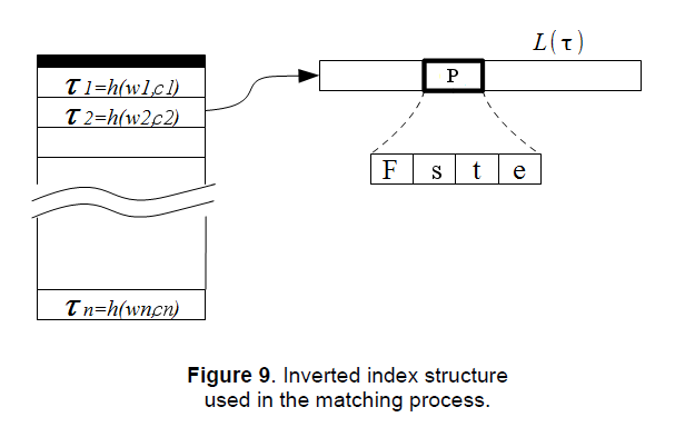
Choosing an appropriate structure to organize the reference database will determine the efficiency of the search algorithm and the scalability of the system. A very popular structure for document retrieval is the inverted index, and we’ll be using this structure in the matching algorithm since the fingerprint model is based on a IR paradigm, so this choice just comes natural.
Inverted indices allow for fast retrieval by using lists of occurrences for each word in the dictionary, called inverted lists. Each occurrence is a small structure, called a posting, containing information about the documents they can be found in, along with supporting information such as the “weight” of the term in the document, the position, etc. In our implementation each posting is a tuple defined as follows
\(P = \langle F,s,t,e \rangle \tag{16}\)
where F is the id of the fingerprint in which the auditory word occurs, s the local fingerprint id, t the time location of the local fingerprint and e the distance of the auditory word associated to s to the word in the dictionary (quantization error). This value will be used as a weight in the similarity measure during the search stage and its role will be clearer in the following sections.
One problem that we faced in the design of the inverted index is the low cardinality of the dictionary. This parameter affects the efficiency of the search when the inverted lists are scanned during the matching stage. In fact, inverted indices work well when the data representation is sparse, that is the number of words occurring in the documents is small compared to the cardinality of the dictionary. The low cardinality of the auditory words set dramatically decreases the sparsity, increasing the size of the inverted lists and, consequently, the processing time during the search stage.
To mitigate this problem we perform a further partitioning of the search space by linearly dividing the spectrum into \(N_{ch}\) frequency channels (we used \(N_{ch}=60\)) and considering the channel where the auditory words occur. The entries in the inverted index will then be as follows
\(\tau_{ic}=w_{i} | c \rightarrow \{P_{1},P_{2},…,P_{m}\},~~~c=1,2,…,N_{ch}~~~i=1,2,…,|W| \tag{17} \)
where \(\tau_{ic}\) indicates the term formed by the concatenation of the i-th auditory word with the c-th channel, as shown in (17). This will increase the size of the partition by 1 order of magnitude from few hundreds to several thousands, giving the inverted index a larger sparsity and, therefore, more efficiency. There are other optimization techniques that can be applied to further increase the efficiency of an inverted index, which can be found in the Information Retrieval literature and are beyond the scope of this paper.
3.2 Candidates search
The indexing structure created in the previous step is used to perform the search of the best matches to a given query. Before describing the matching algorithm, some interesting properties regarding the chosen fingerprint model will be introduced:
1) Time proximity: the local fingerprints in an audio sequence occur all within a defined, bounded and arbitrary time frame, that is
\(\forall w_{i},w_{j} \in X \Rightarrow |t(w_{i})-t(w_{j})| \leq T_{b}\)
where \(T_{b}\) is an arbitrary time interval.
2) Time order: the local fingerprints in an audio sequence, by construction, are ordered in time (and monotonically labeled), that is
\(t(w_{i}) \geq t(w_{j})~~~\forall i>j\)
3) Spatio-temporal coherence: if \(F=\{s_{1},…,s_{n}\}\) is the set of local fingerprints extracted from an audio recording and \(\Psi(F)\) a function describing the spatio-temporal relationships between the local fingerprints in F, then for any two perceptually similar audio \(F_{1}\) and \(F_{2}\) must be \(|\Psi(F_{1})-\Psi(F_{2})|\leq\varepsilon\), with \(\varepsilon\) sufficiently small. That is the relationships between local fingerprints belonging to two matching audio are coherent both in time and frequency.
Considering the above properties, the approach used here to search for candidate matches in the database, that we call time clustering, is similar to the Generalized Hough Transform (GHT). The GHT is a popular method used to detect the presence of known objects (described by their models) within an unknown query by means of a voting scheme in a discretized parameter space (the Hough space). Looking for maxima in this space will reveal the probability of finding the objects of interest. Our GHT-like algorithm uses a matrix \(M_{c}\) called, with a slight abuse of terms, the similarity matrix to capture similarities between the query fingerprint and the reference fingerprints in the database D exploiting property 1) and 2).
Be n the number of fingerprints in D and \(T_{b}\) an arbitrary time step, then the \(m \times n\) matrix \(M_{c}\) can be defined as
\(M_{c}=(F,b)~~~~F=1,2,…,n~~~~b=1,2,…,m\)
where F is the fingerprint index (id) and b the quantized time step given by
\(b=t(w_{F})/T_{b} \tag{18}\)
\(t(w_{F})\) being the time at which word w occurs in fingerprint F . The size of the m dimension depends on the maximum recording duration in D. This matrix will be used in the matching process to segment the search space into regions where finding the best match is highly probable. This is done using the following procedure:
The unknown query sequence \(X=\{x_{1},…,x_{k}\}\) is matched against the dictionary of auditory words built using the binary vector quantization procedure exposed in 2.5. A positive consequence of the low cardinality of the dictionary is that we can perform an exhaustive search on it rather than resort to some kind of approximate nearest neighbor method. The quantization \(w=q(x)\) is performed by comparing each query local fingerprint x to each auditory word w in the dictionary using the Hamming distance as a measure of similarity. The speed of Hamming distance computation, which can be performed using dedicated hardware instructions on modern computers, and the low cardinality of the dictionary makes this process extremely fast. At this point the frequency channels where the words occur are also computed by quantizing their frequency values.
After X is transformed into a sequence of auditory words the search is carried out using the similarity matrix \(M_{c}\) and the inverted index. For each auditory word \(w_{i}=q(x_{i})\) in the query the corresponding inverted list is retrieved, by means of the term index \(\tau_{ic}\) computed as detailed in section 3.1, and the postings processed sequentially. Specifically, for each posting \(P = \langle F,s,t,e \rangle\) in the inverted list \(L(\tau_{ic})\) the cells \(M_{c}(F,b)\) are selected in the similarity matrix, where b is computed as \(b=t/T_{b}\) and a score is assigned according to the following scoring functions
\(S_{tp}(F,b)=\begin{cases} a_{tp} \cdot K_{tp} & \text{if } s \in M_{c}(F,b) \\ 0 & \text{otherwise} \\ \end{cases} \tag{19}\)
and
\(S_{to}(F,b)=\begin{cases} a_{to} \cdot K_{to} & \text{if } t_{i} \geq t_{i-1} ~~~~ s_{i},s_{i-1} \in M_{c}(F,b) \\ 0 & \text{otherwise} \end{cases} \tag{20}\)
These functions assign a similarity score if properties 1) and 2), respectively, are satisfied. Here \(s_{i}\) represents the word in the candidate fingerprint F being selected by \(w_{i}\) at step i, \(K_{tp}\) and \(K_{to}\) are constants, and, \(a_{tp}, a_{to}\) are weights computed as follows
\(\displaystyle a_{tp}=1-\frac{|e_{w}-e|}{|d|} \tag{21}\)
and
\(\displaystyle a_{to}=\frac{n_{o}}{n_{c}} \tag{22}\)
where \(e_{w}\) and \(e\) are the quantization errors of the query word and the word in the candidate fingerprint respectively, \(|d|\) is the size of the descriptor (in bits), \(n_{o}\) the number of candidates satisfying the time order property in the selected matrix cell and \(n_{c}\) the number of candidates in the cell. The total score is then given by
\(S_{TOT}(F,b)=S_{tp}(F,b)+S_{to}(F,b) \tag{23}\)
The idea is to capture similarities between fingerprints by measuring how well property 1) and 2) are satisfied using the above scoring functions. \(S_{tp}\) will give a high score if the time proximity property is satisfied, that is if many local fingerprints for some F in D similar to the query will be localized, while \(S_{to}\) will give a high score if these similar local fingerprints are also temporally ordered. If the query has a corresponding audio or is an excerpt of some audio in the database then it will show very strong similarities in the chosen period of time \(T_{b}\) with some F in D. This will manifest in the matrix as a peak cell indicating a strong correlation that can be used to recognize the best match or to perform further analysis. The weights help in the discrimination and disambiguation during the scoring. The constants \(K_{tp}\) and \(K_{to}\) are set to the same value in our implementation.
For each candidate word that gets clustered in the matrix we also save a list of pairs \(C=\{\langle s,x_{i} \rangle\}\) that will be used at a later stage. Since the scoring procedure is basically a process of integration it is necessary to keep the state between steps in \(M_{c}\). For this purpose, the structure of a cell in \(M_{c}\) holds an accumulator, along with other info, and is defined as follows
\(M_{c}(F,b)=\langle S_{TOT}, t_{s_{i-1}}, n_{o}, C \rangle\)
as shown in Figure 10.

After the query sequence X is processed, the fingerprints corresponding to the k cells in \(M_{c}\) with the maximum scores are the candidate best matches. For large data sets, however, the similarity matrix can become too big to be held in main memory, so to avoid this the matching is done by time row (or column) in a DaaT-fashion using IR terminology, according to the following procedure. Be \(M_{c}(F)=[b_{1},…,b_{m}]\) a row (column) of \(M_{c}\) for some F in D. We denote this row (column) vector by \(H_{F}(b)\) and, since it represents time-related value distributions, we call it a time histogram for F. For each time histogram in \(M_{c}\) find the bin with maximum value \(b_{max}\), that is
\(b_{max}=\underset{b \in [1…m]}{\arg\max}~H_{F}(b) \tag{24}\)
and store the values \(H_{F}(b_{max})\) in a heap. The set of top-k elements in the heap are the candidate matches to the query X. We denote this set by \(D_{C}=\{F_{1},…,F_{k}\}\). It represents a partition of D with a high probability of finding the true match. Depending on the query audio signal, this stage may already be enough to get a clear best match, without the necessity to also verify property 3). Figure 11 shows the state of the similarity matrix during the match of some audio clips on a database of 400 recordings. Clear evidence of a strong similarity can be seen between the queries and the fingerprints 41, 184 and 327 respectively at specific time steps (displayed as bright spots), which happen to be the correct matches.

3.3 Re-ranking
Although in many cases satisfying property 1) and 2) in 3.2 is enough to get a clear best match, as can be seen in Figure 11, it is not always the case that similarities with some fingerprint show so obviously in the similarity matrix. This may occur when there are several recordings in the database that are similar to the query audio or when the quality of the query audio signal is low, in which cases there may be multiple peaks due to false positives. We have noticed that for signals undergoing transformations that are typical in audio production, such as equalization, compression, reverberation, encoding, etc. satisfying only property 1) and 2) is sufficient in many cases without the need for further processing.
However, in more though scenarios, such as heavily distorted signals recorded from noisy environments or using low quality hardware/codecs, the time proximity and time order properties might not impose strict enough constraints and further analysis is required to get a better discrimination. The re-ranking process is performed on the top-k candidates in order to verify property 3). This is done using the set of candidate pairs \(C=\{\langle s_{ij},x_{k} \rangle\}\) in the bins of the time histograms associated with the top-k candidates in the similarity matrix as seeds to perform sequence alignment and graph matching.
Specifically, be \(X^{k}=\{x_{k-\Delta},…,x_{k},…,x_{k+\Delta}\}\) a subsequence extracted from the query sequence centered at \(x_{k}\) and \(G(X^{k},E^{k})\) the fully connected graph having as nodes the local fingerprints in \(X^{k}\) and as edges \(E^{k}\) the position vectors between nodes in the time-frequency space.
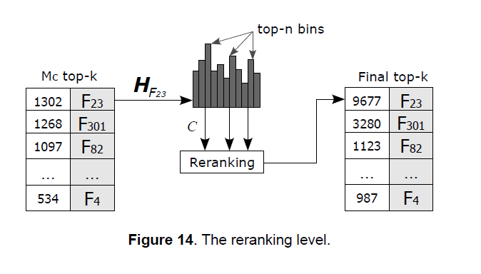
Each query local fingerprint \(x_{k}\) processed in the time clustering stage picks a set of similar local fingerprints belonging to some reference fingerprints in D. These are stored in the cells of the matrix \(M_{c}\) as a set of pairs \(C=\{\langle s_{ij},x_{k} \rangle\}\), where \(s_{ij}\) is the j-th local fingerprint from fingerprint \(F_{i}\) in D. We use the sets C taken from the top-n bins of the time histograms \(H_{F}(b)\) for each candidate in the top-k set \(D_{C}=\{F_{1},…,F_{k}\}\) instead of just from the bin \(b_{max}\) in order to increase the probability of match, as shown in Figure 14. To each query local fingerprint \(x_{k}\) is then associated a set of candidate local fingerprints from the database, as illustrated in the following relation
\(x_{k} \rightarrow C_{k}\{s_{ij}\} \tag{25}\)
Be \(F^{j}=\{s_{i,j-\Delta},…,s_{i,j},…,s_{i,j+\Delta}\}\) a subsequence from the top-k candidate fingerprint \(F_{i}\) centered at \(s_{ij}\), and \(G(F^{j},E^{j})\) the fully connected graph having as nodes the local fingerprints in \(F^{j}\) and as edges \(E^{j}\) the position vectors between them.
Property 3) in 3.2 can then be evaluated by aligning the query sequences \(X^{k}\), determined by the local fingerprints \(x_{k}\), and the candidate sequences \(F^{j}\), determined by the set \(C_{k}\), and matching the graphs \(G(X^{k},E^{k})\) and \(G(F^{j},E^{j})\) using a scoring function \(S_{COH}(G(X^{k},E^{k}), G(F^{j},E^{j}))\), which will be defined later, as depicted in Figure 12.
The \(\Delta\) parameter determines the size of the neighborhoods around the reference local fingerprints to be matched. Since it also determines the size of the graphs its value should not be too high in order to keep the computational cost within acceptable limits. On the other hand, setting a value that is too small may affect the accuracy, so a tradeoff is needed. From our experiments, good values have been found to lie in the range [10, 20].

3.3.1 Graph matching by Pairwise Geodetic Hashing
Graph matching is the process of finding a mapping between the nodes and the edges of two graphs in order to realize a correspondence between similar structures shared by the two graphs. This correspondence can be a one-to-one, in which matching pairs of nodes between the graphs must preserve the edges connecting the nodes (exact graph matching) or a more relaxed form where deformations in the edges are allowed (approximate graph matching). In its naive form this problem is inherently combinatorial, hence computationally expensive, and there are many methods in the literature that tackle the problem from different perspectives in order to reduce its complexity. Our approach uses a similarity function based on Pairwise Geodetic Hashing, an algorithm inspired to the Geometric Hashing technique, to solve the correspondence problem.
Geometric Hashing is a well known technique for object matching introduced in [15] and [16]. The basic idea is to extract geometric features from an object and to index them using a transformation-invariant hashing function in order to capture the geometric relations among such features regardless of the transformation that might have been applied to the unknown object.
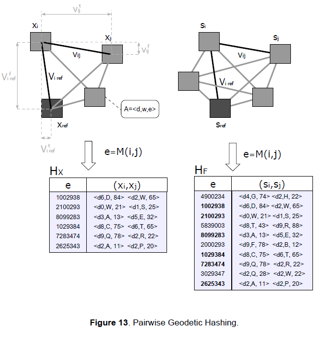
Given two attributed graphs \(G(X^{k},E^{k},A^{k}), G(F^{j},E^{j},A^{j})\) the adjacency matrices \(M_{X}, M_{F}\) can be built so that each element of the matrix represents the position vector v between two local fingerprints. Since the graphs are simple and undirected, these adjacency matrices are symmetrical and triangular, so for a \(n \times n\) matrix we only need to consider \(n(n-1)/2\) elements. These elements can be indexed in a lookup table, where each index is associated to the pair of local fingerprints connected by that position vector, along with some attributes A. The similarity between the graphs can then be quickly computed using these lookup tables by scoring the matching edges and the similarity between the nodes according to the set of attributes. The time and frequency values are quantized to allow some deformation in the graphs and account for errors due to noisy signals.
To disambiguate the edges we pair them to a reference edge represented by the position vector between the local fingerprint being processed and a reference local fingerprint. This reference node should be one that’s common to both the query graphs and the candidate graphs in order for the match to succeed. As reference nodes we then choose the query local fingerprints \(x_{k}\) and the associated candidates \(C_{k}=\{s_{ij}\}\) picked in the time clustering stage. If \(x_{k}\) and \(s_{ij}\) happen to belong to the same fingerprint then the graphs they induce will be constructed using the same reference system and they will match to some degree.
The lookup tables are implemented using hash tables to get O(1) time complexity and have the following structure
\(H[M(i,j)]=(s_{i},s_{j}) \tag{26}\)
where the keys M(i,j) are created by hashing the elements of the adjacency matrix using the following hashing function
\(M(i,j)=v_{ij}^{t} \oplus v_{ij}^{f} \oplus v_{i,ref}^{t} \oplus v_{i,ref}^{f} \tag{27}\)
the \(\oplus\) operator indicates concatenation, \(v_{ij}^{t}\) and \(v_{ij}^{f}\) the time component and frequency component respectively of the position vector between the i-th node and j-th node, \(v_{i,ref}^{t}\) and \(v_{i,ref}^{f}\) the time component and frequency component of the position vector between the i-th node and reference node. These hashed values will be the keys e of the hash table, as depicted in Figure 13.
The scoring is performed by considering both the geometric relationships and the similarity between local fingerprints using specific node attributes according to the following scoring function
\(S_{COH}(G(X^{k},E^{k},A^{k}), G(F^{j},E^{j},A^{j}))=\displaystyle\sum_{e \in E^{k} \cap E^{j}} K_{c} + a_{s}(e) \cdot K_{s} \tag{28}\)
where
\(a_{s}(e)=2-\frac{1}{|d|} [D_{H}(x_{i}^{e},s_{i}^{e})+D_{H}(x_{j}^{e},s_{j}^{e})] \tag{29}\)
For each common edge \(e\), that is the intersection between \(E^{k}\) and \(E^{j}\) which can be computed by finding common keys between the hash tables \(H_{X}\) and \(H_{F}\), the function gives a constant score \(K_{c}\) for the spatio-temporal coherence and a weighed score \(K_{s}\) for the similarity between the local fingerprints connected by the edge. \(D_{H}(x^{e},s^{e})\) denotes the Hamming distance between the query local fingerprint and the candidate local fingerprint at both ends of the common edge \(e\). In our implementation we used the same value for \(K_{c}\) and \(K_{s}\). Note that the nodes attributes in this case coincide with the local fingerprints descriptors but other parameters may be used to measure the similarity, as we’ll see below.
The above similarity function requires the binary descriptors be stored in order to compute the Hamming distance, which can result in high storage space requirements for large datasets. To avoid this, the following similarity function can be used
\(\displaystyle a_{s}(e)=\frac{1}{|d|} [\beta(w_{x_{i}^{e}}, w_{s_{i}^{e}})+\beta(w_{x_{j}^{e}}, w_{s_{j}^{e}})] \tag{30}\)
where \(w=q(x)\) are the auditory words resulting from the binary vector quantization, \(\beta(\bullet,\bullet)\) a function defined as follows
\(\beta(w_{1},w_{2})=\begin{cases} |d|-|\epsilon(w_{1})-\epsilon(w_{2})| & \text{if } w_{1}=w_{2} \\ 0 & \text{if } w_{1} \neq w_{2}\\ \end{cases} \tag{31}\)
and \(\epsilon(w)\) the quantization error of \(w\). This implementation uses simple relational operations instead of the Hamming distance as a measure of similarity and only requires storing the auditory words and their quantization errors (which can be precomputed) rather than the whole descriptors, with massive savings in terms of storage space.
The results of the re-ranking are stored in a final top-k list, as depicted in Figure 14. The effect of the re-ranking process is that of increasing the probability of match in the top-k list when the scores between the candidates are too close.
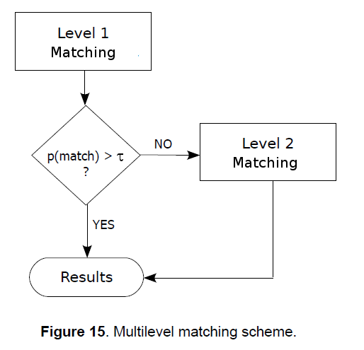
The use of two different scoring systems makes the matching algorithm a multi-level (2-level) process. At the first level is the time clustering scoring which tries to match the unknown query using only a subset of the properties that must be validated (loose matching). If these properties already satisfy the matching condition, then the process stops at the first level, otherwise, it proceeds to the next level, where stricter constraints are used. This approach can be used to make the algorithm adaptive, using computational resources only if necessary. For example, depending on the application, a threshold τ may be adjusted in order to make use of only the first level if the audio is not subject to appreciable distortions, switching off the second level thus saving computational resources, or it may be set so that Level 2 matching only kicks in if the threshold is reached, or it can be set to always perform the Level 2 matching if the application deals with noisy audio. The below diagram depicts the whole concept.
4. Performances
In the following sections we show how we evaluated the performances of the proposed method. The algorithms have been designed with no specific use case in mind and one of the main goals is that of achieving as much generalization power as possible. While our method may be applied to different kind of audio signals by building an appropriate auditory words dictionary using specific training sets, here we only show the results of tests conducted on music contents, since it’s probably the most common application.
The experiments have been carried out using 10,000 query audio clips extracted from a set of 1,000 music recordings of different genres. To test the time-translation-invariance of the fingerprint model the clips were taken at random offsets within the recordings.
4.1. Robustness
In order to verify the robustness of the method we applied various transformations to the query clips that have been typically used to test other audio identification systems and that are listed in Table 1, along with the respective accuracy. The results clearly show the validity of our method in solving audio content identification problems. However, applying single processing steps to audio signals is not very realistic, as in real world scenarios the audio typically undergoes different transformations before being published and/or delivered to the recipients. In this regards, we use different audio models in an attempt to represent different scenarios where ACI technology may be applied.

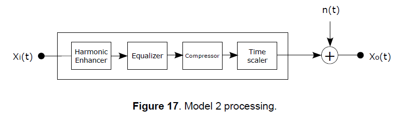
Model 1 represents a scenario where the audio signal is passed through a chain of processing stages with the purpose of altering its characteristics. This is common, for example, in radio broadcasting. The processing chain is not standard and may vary considerably with a wide range of possible settings depending on the application, but after some research it appears that typical processing chains in broadcast audio include stereo wideners to increase the ambience, harmonic enhancers to give the sound a brighter and clearer presence, equalization to emphasize specific aspects of the sound (for example bass, voice or treble enhancing), dynamic range compression to make the sound evenly louder and give it more presence, and, very often, “time stretching” to change the duration of the recordings without altering the pitch (common with commercial broadcasters to increase the advertisement time or keep programs within schedule). In our model we choose the processing chain depicted in Figure 16 with the following settings: for the harmonic enhancer we added even order harmonics at a crossover frequency of 4kHz with a drive of 6dB, the equalization stage applied the EMI 78 curve to emphasize the bass while reducing very high frequencies where noise may be present, the compressor was set with a threshold of -35dB and ratio, attack and release of 6:1, 100ms and 1s respectively, while the tempo was scaled up by 10%.

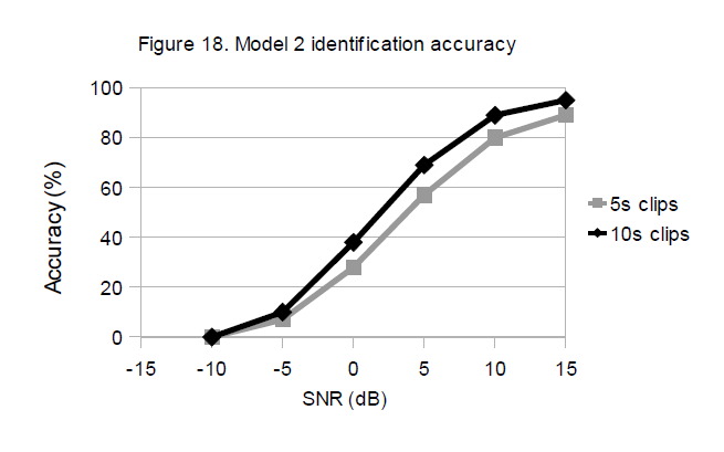
Model 2 represents a tougher scenario where the original audio signal is passed through the processing chain of Model 1 and additively combined to another audio signal. A typical application that can be roughly modeled in this way is ambient audio identification, where preprocessed audio (for example a radio broadcast or other source) is played in an environment and affected by background noise before being recorded by the ACI system. There are of course other factors that the model does not keep into account in similar applications, such as the limited frequency response of low quality speakers (for example if the audio is played by a portable device), the effects of reverberation, the distortions in the recording device, etc. The background noise sample used in the tests was recorded in a marketplace and has been randomly added to the query clips at various Signal to Noise Ratios.
The results for the two models are reported in Table 3. It shows that the proposed method is also effective for recognition of distorted audio in the presence of additive noise (within limits of course). The tests were conducted following a forced-choice approach, that is all the query audio clips were taken from recordings present in the database and the system was forced to choose a best match. We noticed that most of the false positives were for clips that have been taken from parts of the recordings with too few or no audio events (such as transitions, pauses, faded audio, etc.) and for clips with very similar noise-like sounds that would be extremely hard to identify even for the most trained human ear.

4.2 Speed
The responsiveness of a system is a fundamental parameter when it comes to real-time applications so we investigate the identification times by analyzing the key factors that contribute to the overall system’s performance. The recognition time basically depends on the speed of the fingerprinting and matching processes, which have a constant and linear time complexity of \(O(T_{i})\) and \(O(|D|)\) respectively at each processing step, where \(T_{i}\) is the duration of an input audio block (fixed) and \(|D|\) the size of the fingerprint database. Extracting an audio signature from 1 second of audio took approximately 6 ms on average (real-time factor of about 167), while searching the fingerprint space for a match depends on the size of the fingerprint database and the distribution of the words in the index. On a simulated database of 10,000 recordings with an average duration of 5 minutes and a quasi-uniform distribution of words it took on average 210ms to search for a match (real-time factor 4.76). These figures where obtained using hardware-non-optimized algorithms (aside from the FFT computation) written in C++ and running on a laptop computer with a 2.53GHz i5 processor, 3MB L3 cache and 4GB of RAM.
4.3 Compactness
The size of the fingerprints have a determinant role on the performances of a recognition system and a big chunk of the design must be devolved to the implementation of a fingerprint model with the optimal trade-off between accuracy, speed and scalability. Our fingerprinting method is adaptive as it selects the interest points based on the characteristics of the audio, so the granularity is not fixed and depends on the size of the maxima suppression window \(W_{p}\). A rough estimation of the expected number of (local) fingerprints per time unit can be calculated using the following
\(\mu_{LF} \approx \left\lfloor \frac{\Delta T}{\Delta T_{W_{p}}} \right\rfloor \cdot \left\lfloor \frac{\Delta f}{\Delta f_{W_{p}}} \right\rfloor \tag{32}\)
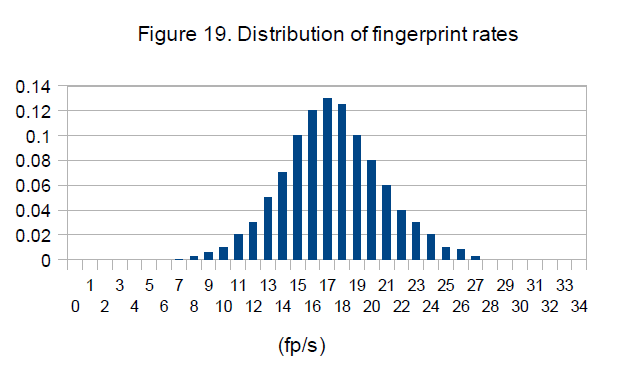 which, with the current settings, corresponds to 18 fingerprints per second. A statistical analysis on the music database used for our experiments reveals that this is indeed the average granularity, as can be seen in Figure 19. Considering that the auditory words are 7-bit binary vectors, the p.d.f. in Figure 19 indicates an average rate of about 18 words per second, that is a mean throughput of 126 b/s. Thus, our method produces very compact fingerprints allowing, for example, a music database of 1 million recordings with an average duration of 4 minutes be fingerprinted using less than 4GB of storage space (excluding support information).
5. Conclusions and further work
We have presented an audio content identification method based on a binary “auditory words” model built using local binary descriptors and inspired to techniques and paradigms from the computer vision and information retrieval communities. Previous works have already shown the efficacy of some methods used for visual recognition to solve audio content identification problems and our work demonstrates how not only specific processing techniques but entire models and paradigms can be adopted. This is a further confirmation of the validity of this approach showing that many techniques, models and paradigms are transferable if a suitable mapping between apparently different worlds is found. Further work should be focused on the search algorithm, particularly on the use of more efficient data structures. Inverted indices may easily become inefficient on very large data sets if no kind of optimization is used, such as early termination, multi-level indexing, list skipping, etc. Fortunately there is a huge amount of research in the IR community on techniques to optimize this data structure, so this is up for future work. A thorough analysis of the parameters of the system (especially those used to build the descriptors) to observe how the variation of these values impact the system’s performances is also worth further investigation.
References
[1] J. Haitsma, T. Kalker. “A Highly Robust Audio Fingerprinting System”, Proc. International Conf. Music Information Retrieval, 2002.
[2] P. Cano, E. Batlle, H. Mayer, and H. Neuschmied. “Robust sound modeling for song detection in broadcast audio”, in Proc. AES 112th Int. Conv., Munich, Germany, May 2002.
[3] Cheng Yang. “MACS: Music Audio Characteristic Sequence Indexing For Similarity Retrieval”, in IEEE Workshop on Applications of Signal Processing to Audio and Acoustics, 2001.
[4] A.Wang. “An industrial-strength audio search algorithm”, in Proc. of International Conference on Music Information Retrieval (ISMIR), 2003.
[5] J. Herre, E. Allamanche, and O. Hellmuth. “Robust matching of audio signals using spectral flatness features”, in Proc. IEEE Workshop on Applications of Signal Processing to Audio and Acoustics (WASPAA), 2001, pp. 127–130.
[6] Y. Ke, D. Hoiem, and R. Sukthankar. “Computer vision for music identification”, in Proc. Int. Conf. on Computer Vision and Pattern Recognition (CVPR), 2005, pp. 597–604.
[7] Shumeet Baluja, Michele Covell. “Content Fingerprinting Using Wavelets”, Proc. CVMP, 2006.
[8] Ramin Zabih1 and John Woodll. “Non-parametric Local Transforms for Computing Visual Correspondence”, in Proceedings of European Conference on Computer Vision, Stockholm, Sweden, May 1994, pages 151-158.
[9] M. Calonder, V. Lepetit, C. Strecha, and P. Fua. “BRIEF: Binary Robust Independent Elementary Features”, in Computer Vision–ECCV 2010, pages 778–792, 2010.
[10] A. Alahi, R. Ortiz, and P. Vandergheynst. “FREAK: Fast Retina Keypoint”, in IEEE Conference on Computer Vision and Pattern Recognition, 2012.
[11] E. Rublee, V. Rabaud, K. Konolige, and G. Bradski. “Orb: An efficient alternative to SIFT or SURF”, in International Conference on Computer Vision, (Barcelona), 2011.
[12] Pasi Fränti, Timo Kaukoranta. “Binary vector quantizer design using soft centroids”, in Signal Processing: Image Communication 14, 1999.
[13] C. Grana, D. Borghesani, M. Manfredi, R. Cucchiara, “A Fast Approach for Integrating ORB Descriptors in the Bag of Words Model”, in press on Proceedings of IS&T/SPIE Electronic Imaging: Multimedia Content Access: Algorithms and Systems, San Francisco, California, US, Feb. 2-7, 2013.
[14] J. Sivic and A. Zisserman. “Video Google: A Text Retrieval Approach to Object Matching in Videos”, in Proceedings of the Ninth IEEE International Conference on Computer Vision, 2003.
[15] Jacob T. Schwartz and Micha Sharir. “Identification of Partially Obscured Objects in Two and Three Dimensions by Matching Noisy Characteristic Curves”, in The International Journal of Robotics Research, 1987.
[16] Y.Lamdan, J.Schwartz, and H.Wolfson. “Affine invariant model-based object recognition”, IEEE Trans. Robotics and Automation, 6:578-589, 1990.
[17] Justin Zobel and Alistair Moffat. “Inverted files for text search engines”, in ACM Computing Surveys, 38(2):6, 2006.
[18] H. Turtle and J. Flood. “Query evaluation: Strategies and optimizations”, in Information Processing and Management, 31(6):831–850, 1995.
[19] M. Fontoura , V. Josifovski , J. Liu , S. Venkatesan , X. Zhu , J. Zien. “Evaluation Strategies for Topk Queries over MemoryResident Inverted Indexes”.