
This article is the first of a series that provides a lean and mean overview of the fundamental principles underlying image filtering. It’s aimed at software developers required to work on image processing projects, and presents practical examples of applications commonly found in this field. The supporting math has been purposely simplified and reduced to the bare bone to avoid complex details that would be of little help to those who are mainly interested in the application aspect of these concepts. To better understand the subject, however, some basic notions of Systems Theory and Digital Signal Processing will be introduced since they’re beneficial (and sometimes necessary) to grasp the workings of this powerful operation. Code examples will also be provided in order to see how these abstract ideas translate into concrete implementations.
Filtering is perhaps the most widely used operation in image processing. In any application involving the manipulation of images, such as computer vision applications, there is some sort of filtering going on somewhere along the pipeline, and often times it is the key factor in the final performances of the system. However, filtering is quite a big subject in the engineering field, supported by complex mathematical concepts that may not be in the background knowledge of many software developers, so it becomes easily intimidating for the “non-practitioner” trying to approach it beyond the mere calling of a library function.
Probably many of you are already acquainted with the concept of filtering in the context of specific applications, such as removing noise from audio or enhance images. Here we start to approach it in the most general way and use the term “filter” broadly to indicate any kind of processing applied to a generic signal to transform it in order to get the desired effects, and then naturally transition to the particular case of digital images.
In general, filtering operations can be classified into 3 categories, depending on how the samples at each point p in the output (filtered) signal y are computed with respect to the input signal x :
- Point filtering: each sample in the output is computed using the value of only one single sample from the input signal, that is \(y(p) = f(x(p))\)
- Local filtering: each sample in the output is computed using the values from a neighborhood N of some point p in the input signal, that is \(y(p) = f(x(N_p))\).
- Global filtering: each sample in the output is computed from the values of all samples in the input, that is \(y(p) = f(x)\)
In these articles we’ll examine solely local filtering operations. Needless to say that we are also only interested in filters that can be implemented in software and executed by a computing device, that is the class of digital filters.
First of all, it is important to know that to get a holistic view of the behavior of a filtering system we need to be able to analyze it in its two domains of existence: the time-space domain and the frequency domain. Many filters that we will discuss later (specifically the linear ones) can be observed in these two domains. The time-space domain is the “natural” domain where many real-world signals are generated and evolve, such as audio signals, electric signals, optical signals, etc. The frequency domain, on the other hand, is a sort of “artificial” domain that allows us to observe a signal under a different light in order to reveal specific characteristics that are not readily apparent in the time-space domain. Understanding both and being able to analyze a signal in either domain is paramount to fully comprehend how filtering works and how to get the most out of its practical applications.
Time-space domain analysis
A filter can be modeled as a system that processes its input signal \(x(\cdot)\), possibly together with some parameters \(\alpha\), to generate an output signal \(y(\cdot)\) by means of a mapping function \(S\), called the system’s function (or the transfer function, even though this term is often used in the literature to indicate the frequency response of the system, so we’ll use this convention here). Fig.1 shows a diagram of a generic filtering system in the time-space domain, where the independent variable (•) represents either time or space.
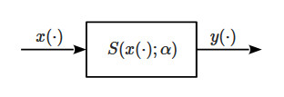
In many cases the system’s function \(S\) has a well defined mathematical expression, but in the digital domain it can also be an algorithm or a complex computer program. Regardless, the output of the system can be written using the following equation
$$ y(\cdot) = S(x(\cdot); \alpha) \tag{1}$$
Although several filters have parameters (e.g. the Gaussian filter), many that we’ll analyze do not, so we’ll often leave out the dependence on \(\alpha\) in the above equation (1) without loss of generality.
Of particular interest is the class of systems called Linear Time/Space Invariant (LTI or LSI depending on what the independent variable represents), which model many real world phenomena and for which there is a vast array of mathematical tools that allow us to study them in detail. We will also consider discrete signals as we’re interested in quantities that can be manipulated and analyzed by a computer, so the independent variable represents sampled points in a specific domain, which for digital images means sampled points in the 2D space.
The terms “Linear Time/Space Invariant” indicate important properties that are crucial to understanding the types of filter that we’ll discuss later, so we’ll give a brief explanation of their meaning. An LT/SI system is linear if and only if its system function fulfills the properties of homogeneity and additivity, that is
$$ \begin{array}{l} 1. & S(kx) = kS(x) \\ 2. & S(x_1 + x_2) = S(x_1) + S(x_2) \end{array} \tag{2}$$
which mean that if the input is scaled by a constant quantity then the output will be scaled by the same quantity as well, and if the input is the sum of two (or more) signals then the output will be the sum of the responses that would be generated if the inputs acted on the system individually. These properties combined define what is known as the superposition principle, that can be written as follows
$$ S(k_1 x_1 + k_2 x_2) = k_1 S(x_1) + k_2 S(x_2) \tag{2.1}$$
Another important consequence of linearity is the possibility of analyzing a filtering problem in the frequency domain, where it can be more efficiently solved. In fact, we’ll see in the next section that all these properties hold true in the frequency domain as well.
Time/space-invariance is a property often found in LT/SI systems (but it’s not necessary for linearity). A linear system is said to be time/space-invariant if its system function does not depend directly on the time (or space) variable. This principle is characterized by the so-called shift-invariance property, defined as follows
$$ \begin{array}{l} 3. & S(x(t)) = y(t) \Rightarrow S(x(t+\tau)) = y(t+\tau) \end{array} \tag{3}$$
which simply means that if the input is shifted by some quantity (in either time or space) then the output will be shifted by the same quantity. In other words, given an input the system generates the same output regardless of when/where it happens (it behaves the same in time/space). All these properties combined have a very important consequence. Specifically, it is possible to show that for any LT/SI system if the input is an impulse \(\delta[n]\) then the system’s response completely describes its dynamics.
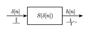
The response function in this case, denoted with \(h[n]\), is called the impulse response of the system, also referred to as the filter or kernel in the image processing world, and knowledge of this function has a very powerful implication. In fact, since it completely characterizes the system, it allows us to know its response to any input signal. In particular, using properties (2) and (3) it can easily be proven that such a response \(y[n]\) is obtained by a linear combination (superposition) of infinite impulse responses, formally defined by the following sum
$$ y[n] = \sum_{i=-\infty}^{\infty} h[i]x[n-i] \tag{4}$$
which is denoted using the following notation
$$ y[n]=(h*x)[n] \tag{4.1}$$
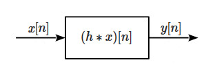
The operation defined in (4) is called convolution and is one of the most powerful mathematical tools in engineering as it allows to know the behavior of an LT/SI system to any input using a simple linear combination with its impulse response. In fact, any LT/SI system can be represented by a convolution operation, as shown in Fig.3. The term “filter” specifically refers to the function \(h\), that can be opportunely designed and applied to any signal using convolution in order to manipulate it and obtain the desired effect. The resulting filter will be, by definition, a linear filter, also called convolution filter (we will use both terms to indicate the same concept).
By looking at equation (4) it can be seen that what convolution does, in a nutshell, is compute the response of the system at some point n as a weighted sum of the impulse response with a reversed version of the input signal (the argument of x runs in the opposite direction as h) in a theoretically infinite interval around n. This operation is repeated for each point n by sliding the filter over the signal (or vice versa, which is the same) until the whole response is computed. In the literature sometimes a slightly different definition of convolution can be found, specified as follows
$$ y[n] = \sum_{i=-\infty}^{\infty} h[i]x[n+i] \tag{4.2}$$
That is technically a cross-correlation and is equivalent to convolution only if the filter is symmetric, in which case reversing it wouldn’t make any difference. Also, the definition of convolution requires signals of infinite lengths, but in real world applications we deal with finite signals. To overcome this issue the sum in (4) can be limited by considering the signals to be zero outside of their intervals of definition so that the convolution is computed only when the signals overlap, and is zero otherwise. This can be better seen with the graphical example in Fig.3.1
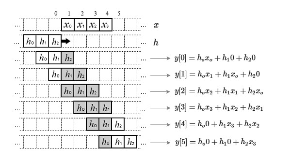
Fig. 3.1 depicts an example of 1D convolution between a signal \(x\) of length 4 and a signal \(h\) of length 3. The signals are overlapped and one of them (\(h\) in this case, but it can be any of them) is slid over the other. At the point when they start overlapping the computation of the output \(y\) begins (usually from point zero) and is repeated for each shift until the signals do not overlap anymore. If \(h\) is of length P and \(x\) of length N, then the resulting output will be of length P + N – 1 (which is equal to 6 in the example of Fig.3.1). This is usually called a “full” convolution as it is computed for each point where the signals overlap. In many cases, however, like in most image processing applications, we want the output signal be of the same length as the input. In this instance, considering for example \(h\) defined in the interval [-a, a] (symmetrical for convenience) we can rewrite (4) as follows
$$ y[n] = \sum_{i=-a}^{a} h[i]x[n-i], \hspace{5pt} n=0,…,N-1 \tag{5}$$
or in the following equivalent form
$$ y[n] = \sum_{i=0}^{P_o} h[i]x[n+a-i] \tag{5.1}$$
where \(P_o=2a\), and \(P=2a+1\) is the size of the filter. Equation (5) yields a “partial” convolution as it truncates the computation generating output signals with equal length as the input signals. It also suffers from “boundary effects” at both ends of the interval (see below for details). Another variant can be obtained by manipulating the indices so that the convolution is only defined when the signals completely overlap, in which case the output would be shorter than the input and there will not be boundary effects. We will consider the form in (5) in the following sections as that’s the most used in image processing.
The practical application of convolution presents a computation issue: since the signals are finite, shifting one over the other will inevitably result in the shifted signal to cross the boundaries of the other. This effect generates a condition of uncertainty, as the signal will overlap missing samples. For example, the convolution as defined in (5) produces a condition of uncertainty, when the filter shifts over the limits, by a maximum amount equal to \(a\). There are several solutions to this issue, but all of them will cause some sort of side effect or distortion in the output signal
- extend the signal by padding with a constant value
- start the convolution at an offset equal to \(a\) (this will result in the convolution with a cropped version of the signal and thus a smaller output)
- repeat the signal as if it was periodic by “wrapping it around”, that is take the first and last \(a\) samples of the signal and add them at the end and beginning respectively
- mirror the signal at both ends, that is take the first and last \(a\) samples of the signal and add them reversed at the beginning and end respectively
- stretch the signal by repeating the values at the boundaries, that is repeat the first and last sample \(a\) times
- ignore the undefined points and only use the samples that fall inside the filter (this is equivalent to padding with 0 but does not require manipulating the signal).
Convolution is a very powerful operation despite its simplicity because, depending on the nature of \(h\), it allows us to manipulate a signal so that it exhibits specific characteristics. To get a clearer idea of how it works, let’s consider a very simple example.
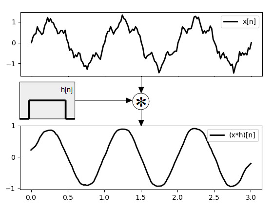
Fig.4 shows a noisy signal \(x[n]\) (top plot), which is a sine wave corrupted by random noise, convolved with a constant filter \(h[n] = 1/11\) defined in the interval [-5, 5]. This convolution basically replaces each point of the original signal with an average of the values in a neighborhood spanning the size of the filter. The result (bottom plot) is a “cleaned up”, smoother version of the original signal. This filter is actually a low-pass filter, also known as “average filter” or “box filter”. Following is an implementation in Python language of the filter in Fig.4.
import matplotlib.pyplot as plt
import math, random

def conv1d(x, h):
    """Naive implementation of 1D convolution"""
    a = len(h) // 2
    y = [0] * len(x)
    for n in range(len(x)):
        for i in range(len(h)):
            p = n + a - i
            if 0 <= p < len(x):
                y[n] += x[p] * h[i]
    return y

def get_x(Tf=3, fs=50):
    """Creates a 1D signal (a noisy sinusoid)"""
    def x(t):
        f = 1
        z = random.uniform(0, 0.5)
        w = 2 * math.pi * f
        return  math.sin(w * t) + z * math.sin(5 * w * t)
    ts = 1 / fs
    N = [n * ts for n in range(0, int(Tf / ts), 1)]
    Xn = [x(n) for n in N]
    return N, Xn

def plot_conv(N, Xn, Yn):
    plt.subplot(211)
    plt.plot(N, Xn, 'k-', linewidth=2, label='x[n]')
    plt.legend()
    plt.subplot(212)
    plt.plot(N, Yn, 'k-', linewidth=2, label='(x*h)[n]')
    plt.legend()
    plt.show()

# A simple average filter
H = [1 / 11] * 11
N, Xn = get_x()
Yn = conv1d(Xn, H)
plot_conv(N, Xn, Yn)
Equation (4) can easily be extended to the 2D discrete space by simply adding an extra dimension to obtain coordinate pairs \([n,m]\) where n indicates the row and m the column number. The two-dimensional (partial) convolution can then be defined as follows
$$\begin{align} y[n,m] & = (h * x)[n,m] \\ & = \sum_{i=-a}^{a} \sum_{j=-b}^{b} h[i,j] x[n – i, m – j] \end{align} \tag{6}$$
or, equivalently
$$\begin{align} y[n,m] & = (h * x)[n,m] \\ & = \sum_{i=0}^{P_o} \sum_{j=0}^{Q_o} h[i,j] x[n+a-i, m+b-j] \end{align} \tag{7}$$
where the upper limits in (7) are given by \(P_o=2a\) and \(Q_o=2b\), while the dimensions of the 2D filter (the kernel’s size) are \(P=2a+1\) and \(Q=2b+1\). The principle is the same as in the one-dimensional case, the only difference being that the linear combinations are performed with a matrix in the 2D space by sliding the kernel in both directions. Fig.5 shows an example where two 2D signals \(h\) and \(x\) of dimensions 3×3 and 5×6 respectively are convolved using (6)
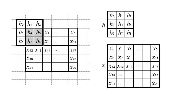
The first pixel’s value in the output \(y[0, 0]\) for the example in Fig.5 is computed with the following linear combination (considering the missing samples to be zero).
$$\begin{aligned} y[0,0] &= \begin{bmatrix} h_0 & h_1 & h_2 \\ h_3 & h_4 & h_5 \\ h_6 & h_7 & h_8 \end{bmatrix} * \begin{bmatrix} 0 & 0 & 0 \\0 & x_0 & x_1 \\ 0 & x_6 & x_7 \end{bmatrix} \\[8pt] &= \begin{aligned} & h_0 \cdot x_7 + h_1 \cdot x_6 + h_2 \cdot 0 + \\ & h_3 \cdot x_1 + h_4 \cdot x_0 + h_5 \cdot 0 + \\ & h_6 \cdot 0 + h_7 \cdot 0 + h_8 \cdot 0 \end{aligned} \end{aligned} \tag{9}$$
Notice how the process mirrors the signal along both dimensions. The very same computation is performed for each sample in \(x\) by shifting the signal \(h\) left to right and top to bottom (or according to whatever the coordinate system is) and the final result is a signal with the same size as \(x\). The boundary effects can be mitigated using one of the solutions described for the 1D case. Linear image filtering is nothing more than applying a filter \(h\) to an image \(g\) to get a processed image \(g_f\) by using (6).
Convolution has some properties that are useful in manipulating expressions where it is used, particularly the following are commonly found in image processing algorithms
$$ \begin{array}{ll} \text{1. Commutativity:} & f * g = g * f \\ \text{2. Associativity:} & f * (g * h) = (f * g) * h \\ \text{3. Scaling:} & k(g*h)=(kg)*h \\ \text{4. Linearity:} & g * (k_1 f_1 + k_2 f_2) = k_1(g*f_1)+k_2(g*f_2) \\ \text{5. Differentiation:} & \nabla (f * g) = \nabla f * g = f * \nabla g \end{array} $$
There are a variety of transformations that can be performed on images by assigning specific values to the kernel’s weights in order to obtain a particular effect, such as removing noise, highlighting details, extracting features, etc. As an example, consider the image g[n,m] and the filter h shown in Fig.5.1. Suppose that for some reason we want the final image to be smoother than the original. One way to achieve this is by convolving g[n,m] with a kernel h where the elements are valued as in Fig.5.1
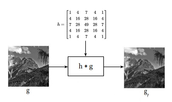
This type of filter is called a Gaussian smoothing filter and we will discuss it in more details in another section. What is important to realize here is that linear filtering is based on the computation of the filtered image by performing a “weighted average” in a neighborhood of each pixel in the original image. The weights, along with their spatial arrangement within the kernel, completely determine the end results. Below is a Python implementation of the filter shown in Fig.5.1
import numpy as np
import cv2 as cv
ipath="/path/to/image"
def conv2d(x, h):
"""Naive implementation of 2D convolution"""
an, am = len(h[0]) // 2, len(h) // 2
N, M = len(x), len(x[0])
I, J = len(h), len(h[0])
y = [[0] * N for _ in range(N)]
def inrange(p):
return (0 <= p[0] < N) and (0 <= p[1] < M)
for n in range(N):
for m in range(M):
for i in range(I):
for j in range(J):
p = (n + an - i, m + am - j)
if inrange(p):
y[n][m] += x[p[0]][p[1]] * h[i][j]
return np.array(y)
h = np.array([
[1, 4, 7, 4, 1],
[4, 16, 28, 16, 4],
[7, 28, 49, 28, 7],
[4, 16, 28, 16, 4],
[1, 4, 7, 4, 1]]) / 289
g = cv.imread(ipath, cv.IMREAD_GRAYSCALE)
gf = conv2d(g, h)
# gf = cv.filter2D(g, -1, h) # using OpenCV
implot([
[(g, "original"), (gf, "filtered")]
])
# Note:
#
# cv.filter2D() actually computes the correlation of
# h with g, not the convolution, but since the kernel
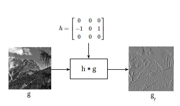
# is symmetric the result is the same.Another example is shown in Fig.5.2 where the image g[n,m] is processed with another type of kernel that highlights specific features, such as edges in a given direction
Convolution in the discrete domain is technically a simple operation (it’s just a sum of products) and it’s fast enough if the filter has a small dimension. However, its computational complexity given an image of size N x M and a kernel of size P x Q is \(O(NMPQ)\), or about \(O(N^2P^2)\) if both dimensions are comparable. This means that the cost of processing an image using convolution quickly increases with the size of the image and kernel. In most applications the kernels are sufficiently small to allow for fast processing, even in real-time, but in other cases the computational cost may be prohibitive and other solutions are necessary, such as performing the filtering in the frequency domain, as we’ll discuss in the next section.
A special case that leads to a more efficient computation of the convolution is when the filter is separable. Generally speaking, a function in an n-dimensional space is said to be separable if it can be decomposed as the product of two functions in lower dimensional spaces. So, a 2D filter is separable if its kernel can be obtained as the product of two vectors. For example, the following kernel is separable
$$ h = \begin{bmatrix} -1 & 0 & 1 \\ -2 & 0 & 2 \\ -1 & 0 & 1 \end{bmatrix} = \begin{bmatrix} 1 \\ 2 \\ 1 \end{bmatrix} \cdot \begin{bmatrix} -1 & 0 & 1 \end{bmatrix} \tag{9.1}$$
In such cases the convolution can be performed in two passes using the two vectors in sequence, that is convolving the image with the column vector first and the row vector afterwards (or viceversa). With this method the computational cost is reduced to \(O(NM(P+Q))\)
Frequency domain analysis
We are already acquainted with signals that vary in time and/or space as it is the natural domain real world phenomena live in. For example acoustic waves, electrical quantities, particle movements, radio waves, are all examples of real world signals that are naturally observed in their temporal and/or spatial progression. However, time and space are not the only domains signals can be observed in, and actually many of their aspects are better studied by ignoring (or augmenting) their dependence on these variables.
For example, often times it is desirable to know which components of a signal are dominant among those that are fast changing and those that are slowly changing. By observing a signal in its time and/or space domain these characteristics are not immediately obvious (if not outright impossible to see). In such cases it would be nice to transform the signal into a different form so that these hidden aspects become evident and can be analytically studied. One such domain is the frequency domain.
To understand the frequency domain analysis, the best way to start is the principle upon which it is based, and that is: any signal can be decomposed into the sum of a (potentially infinite) series of sine waves at opportune frequencies, amplitudes and phases. Transforming the signal into a frequency representation means getting a view at all its sinusoidal components, which are technically known as harmonics. A typical example of this decomposition can be seen in the graphic equalizers found on most digital audio equipment, depicted in Fig.5.3
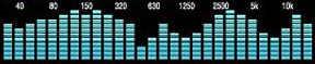
That’s a frequency representation of audio signals across the spectrum of hi-fi music where each bar represents the power of the signal within a given frequency band. So we can clearly see, for example, the bass sounds on the far left, the mid-range sounds (such as vocals) in the middle, and high-pitched sounds (such as percussions) on the far right.
Given a discrete signal \(x[n]\) it is possible to project it to the frequency domain by taking N samples and transforming this sequence using the following equation
$$ X[k] = \sum_{n=0}^{N-1} x[n] e^{-j2 \pi kn/N} \tag{10}$$
The projected signal can be synthesized back to the original domain using the inverse transform, defined as follows
$$ x[n] = \frac{1}{N} \sum_{k=0}^{N-1} X[k] e^{j2 \pi nk/N} \tag{11}$$
where k runs over all the discrete frequencies within the observed period N, that is \(k=0,..,N-1\). The relation (10) is known as the Discrete Fourier Transform (DFT), while equation (11) is called the Inverse Discrete Fourier Transform (IDFT). In the literature, the Fourier Transform (FT) of a signal is usually denoted by \(\mathcal F\{x[n]\}\), and its inverse by \(\mathcal F^{-1}\{X[k]\}\).
The transformed signal \(X[k]\) is generally a series of complex numbers each one representing a sinusoidal component of \(x[n]\) at a discrete frequency with a specific amplitude and phase. These components form the frequency spectrum of the signal and can be used to create different representations such as the power spectrum, the amplitude spectrum, the phase spectrum, etc., by which we can observe aspects of the signal that are not apparent in its original domain and that allow to better understand its dynamics.
Equations (10) and (11) are never directly used in practice for frequency domain analysis as there are more effective methods to compute the FT. Nonetheless, one doesn’t need to be a DSP guru to understand what they do, as they’re so elegant that clearly convey their meaning. In fact, what the DFT does in a nutshell is compare the signal to a set of sinusoids at discrete frequency steps within the observed period N in a sort of correlation of the signal with predefined “sinusoidal templates” (the complex exponential \(e^{jx}\) can be written in terms of sinusoids using Euler’s formula), thus indicating how much of those frequencies are present in the signal. And the IDFT does exactly the inverse, that is given a set of sinusoids at different frequencies it finds the corresponding time domain signal matching that representation.
The FT has several interesting properties that can be used when transforming and manipulating signals in the frequency domain. Here we will only mention a few that are useful in understanding its application to linear filters. Specifically, the FT is a linear operator, that is
$$ \mathcal F_k\{ax_1[n]+bx_2[n]\} = a \mathcal F_k\{x_1[n]\}+b \mathcal F_k\{x_2[n]\} \tag{12.1}$$
A property that is of extreme importance in the design of efficient linear digital filters is that the convolution of two signals in the time-space domain becomes a simple point-to-point multiplication in the frequency domain. This is also known as the convolution theorem and is expressed in the following form
$$ \mathcal F_k\{x_1[n] * x_2[n]\} = X_1[k] \cdot X_2[k] \tag{12.2}$$
For real signals, the FT is symmetrically conjugated and the following relation holds
$$ \mathcal F_k\{x[n]\} = X[k] = \mathcal F_{-k}\{x[n]\} = X[-k] \tag{12.3}$$
Another interesting property is related to the impulse signal \(\delta[n]\), for which it can be shown that the FT is a unitary constant, that is
$$ \mathcal F_k\{\delta[n]\} = 1 \tag{12.4}$$
One of the biggest advantages of linear filters is that they can be analyzed in the frequency domain using the FT. We have seen that any LT/SI system can be represented by convolution with its frequency response and now we want to project that model to the frequency domain. This can be accomplished by transforming the signals using the FT so that we have the frequency represention of a linear filter depicted in Fig.6
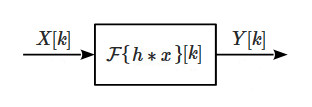
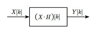
where the independent variable k is the discrete frequency within the considered period N, \(X[k]\) the FT of the input signal, \(\mathcal F\{h * x\}[k]\) the FT of the system’s function, and \(Y[k]\) the response of the system. By applying property (12.2) the convolution operation becomes a point-wise multiplication between the input signal and the filter’s impulse response, so the system’s function of a linear filter in the frequency domain is a simple product between two signals (albeit complex-valued) (Fig.7)
Now consider a generic filter \(H[k]\) and apply to the input an impulse \(\delta[n]\). Then, using property (12.4), the response of the system will be given by
$$ \begin{align} Y[k] &= X[k] \cdot H[k] \\ &= \mathcal F\{\delta[n]\}[k] \cdot H[k] \\ & = H[k] \end{align} \tag{13}$$
that is, when the filter is given an impulsive input, as a response we get its impulse response, which is typically called the transfer function, or frequency response as it completely characterizes the system in the frequency domain. This is in accordance with what we have already seen in the time domain and, together with all the other results, demonstrates the duality between the frequency and time-space domain, that is they are different views of the same phenomenon.
Let’s see how these concepts apply to real-world examples. Consider the signal in Fig.8 representing an oscillating voltage with two sinusoidal components at frequencies of 4Hz and 7Hz.
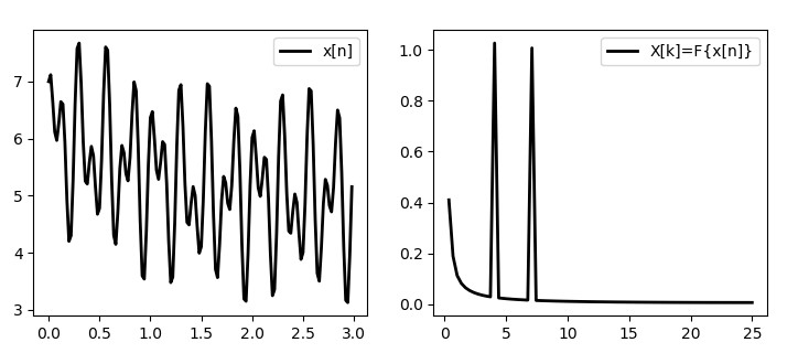
By looking at the time domain representation it is not immediately obvious the nature of these frequency components. By transforming the signal into the frequency domain we can clearly see the presence of the two sinusoids at frequencies 4Hz and 7Hz. Note that the frequency spectrum, in general, spans across both negative and positive frequencies. For real signals, however, the spectrum is symmetric, that is the positive and negative frequencies provide the same information, so usually we only take the positive half. Following is the Python code for the 1D Fourier Transform in Fig.8 using both the plain equations and the Numpy implementation.
import math, cmath
import numpy as np
import matplotlib.pyplot as plt

def dft(x):
    """Compute the 1D DFT using the definition"""
    N = len(x)
    Xn_r = range(N)
    Xk = [complex() for _ in Xn_r]
    for k in Xn_r:
        for n in Xn_r:
            w = 2 * math.pi * k * n / N
            Xk[k] += x[n] * cmath.exp(-1j * w)
    return Xk

def idft(X):
    """Compute the 1D IDFT using the definition"""
    N = len(X)
    X_r = range(N)
    Xn = [complex() for _ in X_r]
    for n in X_r:
        for k in X_r:
            w = 2 * math.pi * k * n / N
            Xn[n] += X[k] * cmath.exp(1j * w)
        Xn[n] /= N
    return Xn

def spectrum(X, fs=50):
    """Create the magnitude spectrum"""
    N = len(X)
    S = [abs(k) / (N/2) for k in X]
    S2 = S[1:N // 2]
    fk = [((k + 1) / len(S2)) * (fs/2) for k in range(len(S2))]
    return fk, S2

def get_x(Tf=3, fs=50):
    """Generate the signal"""
    def x(t):
        dc = 5
        f1, f2 = 4, 7
        w1, w2 = 2 * math.pi * f1, 2 * math.pi * f2
        return  dc + math.sin(w1 * t) \
                   + math.cos(w2 * t) \
                   + math.exp(-t ** 2)
    ts = 1 / fs
    N = [n * ts for n in range(0, int(Tf / ts), 1)]
    Xn = [x(n) for n in N]
    return N, Xn

def plot():
    ax = plt.subplot(311)
    ax.plot(n, Xn)
    ax.set_xlabel("t")
    ax.set_title("signal")
    ax = plt.subplot(312)
    ax.plot(fk, S)
    ax.set_xlabel("Hz")
    ax.set_title("magnitude spectrum")
    ax = plt.subplot(313)
    ax.plot(n, IFXn)
    ax.set_xlabel("t")
    ax.set_title("inverse DFT")
    plt.tight_layout()
    plt.show()

n, Xn = get_x()
FXn = dft(Xn)
fk, S = spectrum(FXn)
IFXn = idft(FXn)
plot()
using Numpy
n, Xn = get_x()
N = len(Xn)
ts = 1 / 50
FXn = np.fft.fft(Xn)
S = np.abs(FXn)
fk = np.fft.fftfreq(N, d=ts)
fk, S = fk[1:N // 2], S[1:N // 2]
IFXn = np.fft.ifft(FXn)
plot()
The 1-dimensional FT defined by equations (11) and (12) can be naturally extended to multivariate signals. In particular, the 2-dimensional DFT is defined by equation (14)
$$ X[k,l] = \sum_{n=0}^{N-1} \sum_{m=0}^{M-1} x[n,m] e^{-j2 \pi (kn/N+lm/M)} \tag{14}$$
from which its IDFT is easily derived
$$ x[n,m] = \frac{1}{NM} \sum_{k=0}^{N-1} \sum_{l=0}^{M-1} X[k,l] e^{j2 \pi (kn/N+lm/M)} \tag{15}$$
Again, these raw equations will never be used in practice as there are more efficient ways of computing the DFT using “fast” algorithms (found in any DSP library). Fig.9 shows the same signal of Fig.8 in two dimensions along with its DFT plotted as a map, which is typical of image analysis. As with the 1-dimensional DFT, the resulting frequency spectrum is symmetric if the input is real (as images typically are).
The centre of the spectrum image represents the zero-frequency component (aka the “dc component”) and the frequency values are increasing in both directions outwards on the k, l axes, that is they’re lower going towards the centre and higher towards the borders. This means that features with slowly changing intensity (such as the sky, the walls of buildings, the skin, etc.) lie around the centre, while features with highly changing intensity such as edges, textures, etc. lie far from the centre.
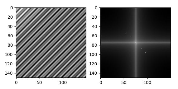
In the example of Fig.9 are clearly visible the two dominant frequency components marked by two bright spots (actually four since their symmetric are also shown) on the diagonal direction, which represents the direction of highest spatial frequency. However, real-world images don’t have such regular structure and present instead more random patterns, as can be seen in. Fig.10.
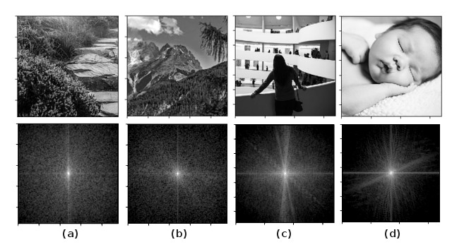
Generally, highly textured images, such as 10(a) and 10(b), have frequency components distributed across the whole spectrum and the respective FTs appear as a noisy pattern, while pictures with more uniform features, such as 10(c) and 10(d), have more low frequency components that show up as a brighter halo concentrated around the centre. It is also interesting to see how the directions of highest intensity variations are clearly visible in images with regular patterns, such as 10(c), and are often associated with the orientation of objects in the scene, even though it’s generally impossible to know which object of the original image as spatial information is lost in the spectrum.
Let’s put all the concepts that we have discussed about time/frequency domain filtering in practice with a more real example. Suppose we have an N x M image g[n,m] that we want to filter in the frequency domain. The first step is to transform it into its frequency representation G[k,l] using the DFT. Then we know that linear filtering in the frequency domain is done by multiplying the image with a suitable kernel H to get the desired effect. The multiplication is performed point-wise, so the kernel H must be a matrix of the same size as the image (this can be achieved by padding the kernel). Remember that the FT of an image is represented by its 2-D spectrum, so filtering an image in the frequency domain means conveniently manipulating the spectrum in order to achieve the wanted results.
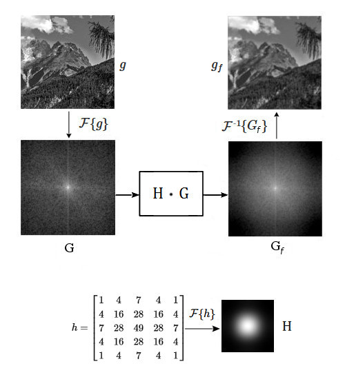
In Fig.11 we are filtering the same image used in the example of Fig.5.1 with the same filter h. However, now we are working in the frequency domain so the filter h is represented by its FT H, which has the spectrum depicted in Fig.11. Once all the signals have been transformed, the filtered image \(G_f\) is computed by multiplying G with H and the resulting image in the spatial domain \(g_f\) is obtained by applying the IDFT to \(G_f\). An implementation in Python is provided below
import numpy as np
import cv2 as cv
import matplotlib.pyplot as plt

ipath="/path/to/image"

def pad(A, B, padder=0):
    """Pad the array A to the dimensions of B"""
    return np.pad(A, ((0, B.shape[0] - A.shape[0]),
                      (0, B.shape[1] - A.shape[1])),
                      'constant', constant_values=padder)

def plot():
    ax = plt.subplot(231)
    ax.imshow(g, cmap='gray')
    ax.set_title("original image")
    ax = plt.subplot(232)
    ax.imshow(pad(h, g), cmap='gray')
    ax.set_title("filter")
    ax = plt.subplot(233)
    ax.imshow(np.abs(gf), cmap='gray')
    ax.set_title("filtered image")
    ax = plt.subplot(234)
    ax.imshow(np.log(np.abs(np.fft.fftshift(G))), cmap='gray')
    ax = plt.subplot(235)
    ax.imshow(np.log(np.abs(np.fft.fftshift(H))), cmap='gray')
    ax = plt.subplot(236)
    ax.imshow(np.log(np.abs(np.fft.fftshift(Gf))), cmap='gray')
    plt.tight_layout()
    plt.show()

h = np.array([
         [1,  4,  7,  4, 1],
         [4, 16, 28, 16, 4],
         [7, 28, 49, 28, 7],
         [4, 16, 28, 16, 4],
         [1,  4,  7,  4, 1]]) / 289

g = cv.imread(ipath, cv.IMREAD_GRAYSCALE).astype(np.float32)

H = np.fft.fft2(pad(h, g))
G = np.fft.fft2(g)
Gf = H * G
gf = np.fft.ifft2(Gf)

plot()
As a side note, the filter in Fig.11 is a low-pass filter as it attenuates the high frequency components (regions with highly varying intensity) resulting in a smooth blurred image. This can be deduced by looking at the spectrum of the filter H that has a shape designed so that when multiplied with the spectrum of the image G the low frequencies around the centre within the cutoff frequency (the radius of the circle) are retained while the high frequencies that lie outside are suppressed.
Filtering in the frequency domain can bring dramatic benefits in terms of computational speed if the filter h is large. For small kernel sizes the convolution is usually more efficient.
Conclusion
There is much more to this subject than the basic concepts exposed in this article, which have been deliberately simplified to avoid as much as possible the complex mathematics behind the theory of filters and DSP in general. The purpose of this article is, after all, not that of giving rigorous mathematical background to the discussed arguments, but rather that of explaining from an engineering point of view how such concepts translate into practical applications. Hopefully these fundamental notions will help developers who are involved in image processing projects but who have minimal or no background in this subject to better understand the principles behind the manipulation of images using digital filters.