
Linear smoothing filters are a specific subclass of linear filters and as such they enjoy all the properties of this class, that is they can be applied using simple linear operations, can be analyzed in the frequency domain and, often, can be efficiently implemented. An introduction to the basic principles of the theory of linear filtering that will allow a better understanding of the concepts discussed in the following sections can be found in the article Fundamentals of image filtering.
Smoothing filters are generally used to level out regions with highly varying intensity that are either generated by destructive processes (e.g. noise) or that are integral part of the image (e.g. edges, fine textures). Depending on how the weights are valued and spatially arranged within the kernel, several types of linear smoothing filters can be defined. We’ll discuss some of the most commonly used along with their characteristics and applications.
Box filter
The box filter is a convolution smoothing filter where the elements of the kernel are uniformly distributed and arranged in a rectangular shape (called the support).
The kernel of a box filter is very simple and is defined by a matrix with all constant values, as follows
$$ h = k \begin{bmatrix} 1 & 1 & \cdots & 1 \\ 1 & 1 & \cdots & 1 \\ \vdots & \vdots & \ddots \\ 1 & 1 & \cdots & 1 \end{bmatrix} \tag{1}$$
where the constant \(k\) is a normalization factor. In practice, it is common to use the sum of the weights (that is the kernel’s size) as a normalization factor
$$ h =\dfrac{1}{p \cdot q} \begin{bmatrix} 1 & 1 & \cdots & 1 \\ 1 & 1 & \cdots & 1 \\ \vdots & \vdots & \ddots \\ 1 & 1 & \cdots & 1 \end{bmatrix} \tag{1.1}$$
where \(p\) and \(q\) represent the size of the kernel in both dimensions. This will ensure that the resulting pixel values are within the dynamic range of the signal. For convolution filters these sizes are usually equal, that is \(p=q=m\). Note that for \(k=1\) the filter computes the integral of the image at the considered pixel.
The box filter (1.1) basically computes each pixel in the resulting image as the arithmetic mean of the pixels within a neighboroud of size \(m\) in the original image. For such reason they are also known as “average filters”. Typical box filters used in applications are shown below
$$ \dfrac{1}{9} \begin{bmatrix} 1 & 1 & 1 \\ 1 & 1 & 1 \\ 1 & 1 & 1 \end{bmatrix}, \hspace{10pt} \dfrac{1}{25} \begin{bmatrix} 1 & 1 & 1 & 1 & 1 \\ 1 & 1 & 1 & 1 & 1 \\ 1 & 1 & 1 & 1 & 1 \\ 1 & 1 & 1 & 1 & 1 \\ 1 & 1 & 1 & 1 & 1 \\ \end{bmatrix} \tag{1.2}$$
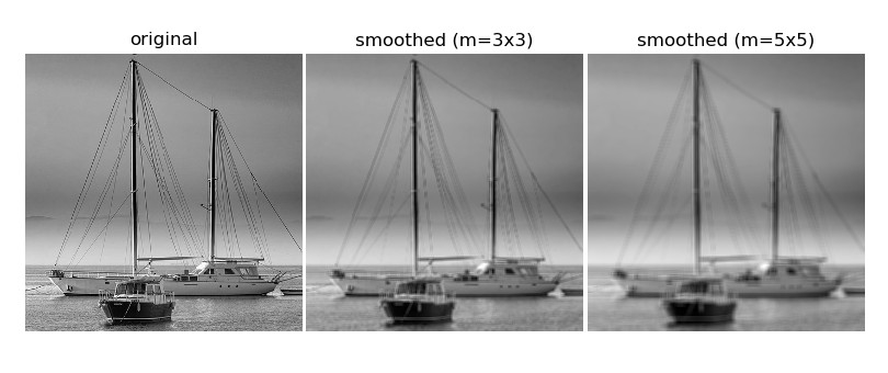
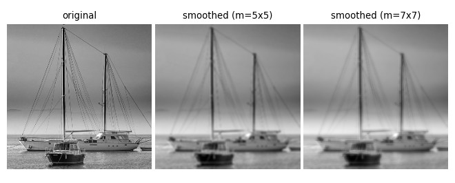
Fig.2 shows some examples of response of the box filter using the kernels defined in (1.2). The central image was smoothed with the kernel of size 3×3, while the one on the right hand side with the kernel of size 5×5. The effect of smoothing filters is that of producing blurred images, and this effect increases with the kernel size since more pixels that may be very uncorrelated to the local features are included in the average.
import numpy as np
import cv2 as cv
import matplotlib.pyplot as plt
ipath="/path/to/image"
h3 = np.array([
[1, 1, 1],
[1, 1, 1],
[1, 1, 1]]) / 9
h5 = np.array([
[1, 1, 1, 1, 1],
[1, 1, 1, 1, 1],
[1, 1, 1, 1, 1],
[1, 1, 1, 1, 1],
[1, 1, 1, 1, 1],]) / 25
g = cv.imread(ipath, cv.IMREAD_GRAYSCALE).astype(np.float32)
gf3 = cv.filter2D(g, -1, h3)
gf5 = cv.filter2D(g, -1, h5)
implot([
[(g, "original"),
(gf3, "smoothed (m=3x3)"),
(gf5, "smoothed (m=5x5)")]
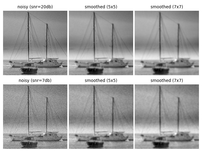
])The most common use case for box filters (as with any other smoothing filter) is for the reduction of noise, so it’s interesting to see its response to noisy images. We will corrupt the original image shown in Fig.2 with noise and analyze the effects of the smoothing with this type of filter. The results are shown in Fig.4.
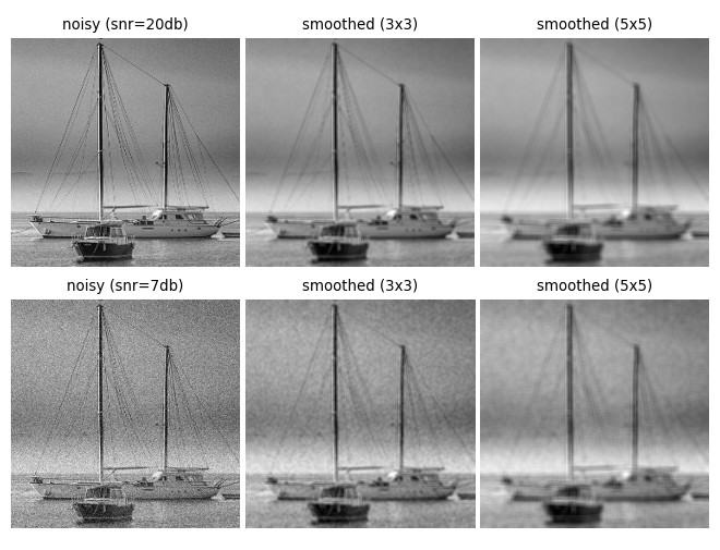
The first row shows the original image corrupted with additive Gaussian noise at SNR 20dB and processed with the box filters (1.2). As can be seen, the noise has been substantially reduced by the smaller 3×3 kernel and almost completely removed by the 5×5 kernel. However, the details of the image have been degraded or wiped out by the blurring effect. Box filters, in fact, treat all pixels in the processed area equally, including those that may not represent the local features, so everything gets leveled out .
The second row shows the same image corrupted with a stronger noise (SNR = 7dB) and then filtered with the same kernels. Even though the noise has been reduced it is still visible in all the filtered images. From these tests it’s evident how the size of the kernel is directly related to the capability of the filter to reduce the noise levels. Specifically, as the noise increases in magnitude, the only way to suppress it is by using bigger kernels, with the consequence of producing a much more blurred image. Following is the Python code used for Fig.4
import numpy as np
import cv2 as cv
import matplotlib.pyplot as plt

ipath="/path/to/image"

def ksnr(s, no, snr):
    """Computes the scaling factor for a given SNR"""
    return np.sqrt(np.sum(s**2) / (10**(0.1 * snr) * np.sum(no**2)))

h3 = np.array([
    [1, 1, 1],
    [1, 1, 1],
    [1, 1, 1]]) / 9

h5 = np.array([
    [1, 1, 1, 1, 1],
    [1, 1, 1, 1, 1],
    [1, 1, 1, 1, 1],
    [1, 1, 1, 1, 1],
    [1, 1, 1, 1, 1],]) / 25

g = cv.imread(ipath, cv.IMREAD_GRAYSCALE).astype(np.float32)
n = np.random.normal(size=g.shape)
g /= 255.0
n = (n - n.min()) / (n.max() - n.min())

kn = ksnr(g, n, 20)
gn1 = g + kn * n

kn = ksnr(g, n, 7)
gn2 = g + kn * n

gn1_3 = cv.filter2D(gn1, -1, h3)
gn1_5 = cv.filter2D(gn1, -1, h5)
gn2_3 = cv.filter2D(gn2, -1, h3)
gn2_5 = cv.filter2D(gn2, -1, h5)

implot([
    [(gn1, "noisy (snr=20db)"),
    (gn1_3, "smoothed (3x3)"),
    (gn1_5, "smoothed (5x5)")],
    [(gn2, "noisy (snr=7db)"),
    (gn2_3, "smoothed (3x3)"),
    (gn2_5, "smoothed (5x5)")]
])
All in all the box filter does a decent job at reducing Gaussian noise, but there are a few problems. As mentioned earlier, the uniform distribution gives the same weight to all the pixels in the neighborhood regardless of their distance from the central pixel. This means that pixels that are far away and that may be loosely correlated to those near the central one will still give the same contribution as those that are very close. As a result, unrepresentative pixels with very high (or low) luminosity can heavily affect the final computation producing strong blurring and distortion of local details.
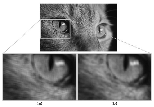
An example of how box filters introduce distortions in images is shown in Fig.3. The image has been processed with a box filter with size 5×5 and the close up (a) highlights a particular region affected by such irregularities.

By looking closely it is possible to notice the presence of vertical and horizontal bands, an effect often referred to as ringing, that generate a “boxy” pattern. The cause is the discontinuity of the uniform distribution at the edges. This discontinuity produces oscillations in the frequency response of the filter, more specifically in its stop-band, with the consequence that high frequencies are not correctly reduced. In the spatial domain this manifests with the irregular smoothing pattern that can be observed in Fig.3. We’ll see this in more details later in this section and it will be more apparent when the same image of Fig.3 is compared to another filter that performs better.
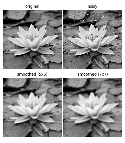
Box filters are not well suited to regularize images with impulsive noise, such as “salt & pepper” noise, because of the excessive contrast with the surrounding pixels, which cannot be eliminated with a linear operation without heavily compromising the details of the image, as can be seen in the following Fig.5

The noisy image has been processed using the kernels (1.2). It can be seen how, although the smaller 3×3 filter has reduced the noise, it is still quite evident throughout the image. The 5×5 filter is able to reduce it further but not completely. In fact, on a closer look it is possible to see the halos left by the averaging process, especially in the brighter areas. Furthermore, the details of the image have been heavily blurred. A bigger kernel would probably reduce it to levels where it’s no longer noticeable but the image would become extremely blurred and the details completely lost. We’ll see in another article how this type of noise can only be effectively removed with non-linear operations. Following is the Python code used for the test in Fig.5
import math, random as rng
import numpy as np
import cv2 as cv
import matplotlib.pyplot as plt

ipath="/path/to/image"

def spnoise(dim):
    """Generate a salt&pepper type of noise"""
    def pdf(gamma=1):
        """Cauchy-Lorentz distribution"""
        dens = 5
        gain = 100
        u = rng.random()
        u = u if u != 0.5 else 0.49
        v = gamma * math.tan(math.pi * u)
        return gain * v if abs(v) <= 1/dens else 0

    return np.array([[pdf(0.01) for _ in range(dim[1])]
                                 for _ in range(dim[0])])

h1 = np.array([
    [1, 1, 1],
    [1, 1, 1],
    [1, 1, 1]]) / 9

h2 = np.array([
    [1, 1, 1, 1, 1],
    [1, 1, 1, 1, 1],
    [1, 1, 1, 1, 1],
    [1, 1, 1, 1, 1],
    [1, 1, 1, 1, 1],]) / 25

g = cv.imread(ipath, cv.IMREAD_GRAYSCALE).astype(np.float32)
n = spnoise(g.shape)
g /= 255.0
kn = 1
gn = np.clip(g + kn * n, 0, 1)
gf1 = cv.filter2D(gn, -1, h1)
gf2 = cv.filter2D(gn, -1, h2)

implot([
    [(g, "original"), (gn, "noisy")],
    [(gf1, "smoothed (3x3)"), (gf2, "smoothed (5x5)")]
])
An interesting property of the box filter is that it is separable, that is it can be decomposed in the product of two orthogonal vectors (a column vector and a row vector) of size \(m\), which allows to reduce the computational cost in the calculation of the convolution.
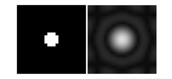
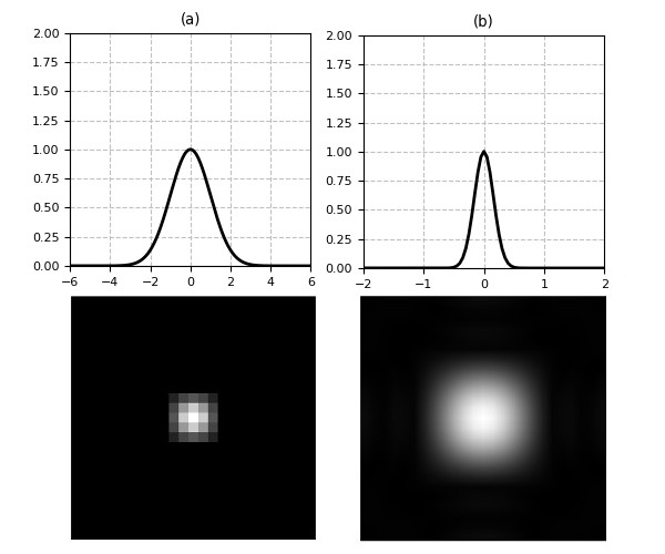
To better understand the characteristics of this filter and why it behaves the way it does we need to analyze its frequency response, which is depicted in Fig.6 as the magnitude spectrum in one and two dimensions.
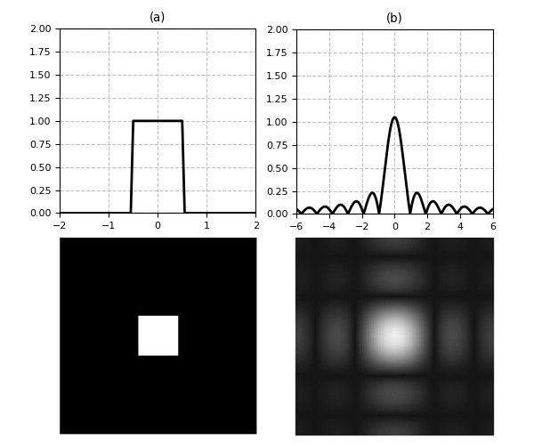
A box filter, as all linear smoothing filters, basically acts like a low-pass filter, as can be seen from its frequency response in Fig.6(b) where the main lobe represents the pass-band. It is evident from the figure that the response of the box filter is not well-behaved as the stop-band is not flat but presents ripples, which are caused by the sharp edges (discontinuities) of the filter in the spatial domain. This effect is known as the Gibbs phenomenon, and can be observed in both the 1D and 2D spectrum (remember that in the 2D spectrum the low frequencies are close to the centre). As a consequence, there will be high frequency components that will leak through the ripples, and since most of the details in images lie in the high end of the spectrum, we can observe these leakages as feature distortions.
Circular filter
The circular filter (aka “pillbox” filter) is a type of uniform filter with the weights arranged into a circular support, as illustrated in Fig.6.1
An interesting property of this filter is its isotropy, that is the smoothing effect is the same in all directions. Following are some examples of circular kernels
$$ \dfrac{1}{5} \begin{bmatrix} 0 & 1 & 0 \\ 1 & 1 & 1 \\ 0 & 1 & 0 \end{bmatrix}, \hspace{10pt} \dfrac{1}{21} \begin{bmatrix} 0 & 1 & 1 & 1 & 0 \\ 1 & 1 & 1 & 1 & 1 \\ 1 & 1 & 1 & 1 & 1 \\ 1 & 1 & 1 & 1 & 1 \\ 0 & 1 & 1 & 1 & 0 \\ \end{bmatrix} \tag{2}$$
The frequency response is depicted in Fig.6.2 and shows how it also suffers from the same issues affecting its boxy sibling.
The results of this type of filter are very similar to those of the box filter, with slightly less (barely noticeable) blurring effects. But unlike box filters, uniform circular filters are not separable and therefore cannot be implemented as efficiently.
Triangular filter
Another variant of average filter is the triangular filter. Its weights are not uniformly distributed as the idea is that of assigning them according to the corresponding pixel’s distance to the centre, with the central pixel having the bigger weight and all the others monotonically decreasing values.
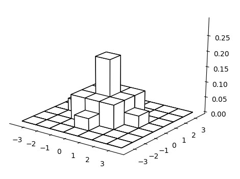
The weights can be arranged into a square (pyramidal) or circular (conical) support, as shown in the following examples
$$ \dfrac{1}{16} \begin{bmatrix} 1 & 2 & 1 \\ 2 & 4 & 2 \\ 1 & 2 &1 \end{bmatrix}, \hspace{10pt} \dfrac{1}{25} \begin{bmatrix} 0 & 0 & 1 & 0 & 0 \\ 0 & 2 & 2 & 2 & 0 \\ 1 & 2 & 5 & 2 & 1 \\ 0 & 2 & 2 & 2 & 0 \\ 0 & 0 & 1 & 0 & 0 \\ \end{bmatrix} \tag{3}$$
Triangular filters perform a weighted average of the pixels with the effect of decreasing the feature distortions typical of uniform filters. Fig.7 shows the results produced by triangular filters using the kernels (3) on the same image used for the box filter

The weighted average makes sure that uncorrelated pixels that are far from the central one contribute minimally to the final computation. The consequence is a diminished blurring effect and better preservation of details compared to the other average filters. The characteristic of this filter can be better seen in the frequency domain, shown in Fig.8 (b)
Compared to box filters, the triangular filter behaves much better as a low-pass because the ripples in its frequency response are more attenuated, thus limiting high frequency leakages and introducing less distortions. Despite its superior results that make it a better choice in many applications over the box filter, it is in general not separable (only those with square support are) so it cannot be as efficiently implemented in all cases.
Gaussian filter
The Gaussian filter is a convolution smoothing filter where the kernel weights are taken from a Gaussian distribution. For a zero-mean distribution with assigned variance \(\sigma^2\) the Gaussian is given by the following function
$$ h(i,j) = k e^{-\frac{i^2+j^2}{2 \sigma^2}} \tag{4}$$
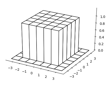
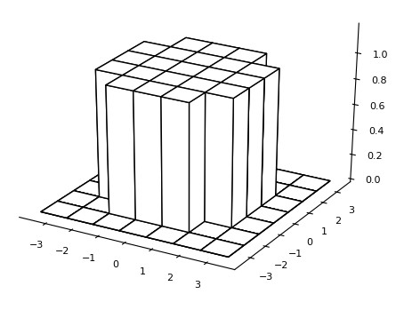
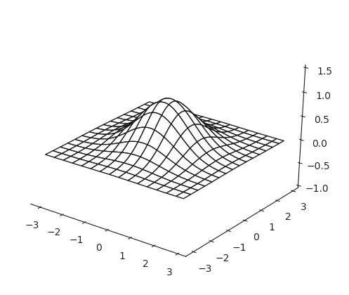
where the \(\sigma\) parameter controls how the weights are distributed in the kernel and determines the “smoothing strength” of the filter, and \(k\) a constant used to normalize the function. Fig.9 shows a 2D Gaussian with zero mean and \(\sigma=1\)
In order to be used with digital images, however, the Gaussian must be discretized with a process of sampling and quantization so that it can be approximated into the finite support of a kernel. Following are two examples of Gaussian kernels for \(\sigma = 1.4\) and \(\sigma = 2\)
$$ \frac{1}{115} \begin{bmatrix} 2 & 4 & 5 & 4 & 2 \\ 4 & 9 & 12 & 9 & 4 \\ 5 & 12 & 15 & 12 & 5 \\ 4 & 9 & 12 & 9 & 4 \\ 2 & 4 & 5 & 4 & 2 \end{bmatrix}, \hspace{10pt} \frac{1}{104} \begin{bmatrix} 1 & 1 & 2 & 2 & 2 & 1 & 1 \\ 1 & 2 & 2 & 4 & 2 & 2 & 1 \\ 2 & 2 & 4 & 8 & 4 & 2 & 2 \\ 2 & 4 & 8 & 16 & 8 & 4 & 2 \\ 2 & 2 & 4 & 8 & 4 & 2 & 2 \\ 1 & 2 & 2 & 4 & 2 & 2 & 1 \\ 1 & 1 & 2 & 2 & 1 & 1 & 1 \end{bmatrix} \tag{5}$$
The results produced by this filter can be observed in Fig.10 where the same original image used for the previous examples has been processed using the kernels (5).
The Gaussian filter has a series of properties that collectively make it a better choice over many other linear filters. First of all, it is isotropic, meaning that its smoothing effect is the same in any direction. In other words, it’s rotation-invariant and works equally well regardless of the orientation of the image.
It performs a weighted average in a circular neighborhood around the central pixel giving each pixel a weight that’s inversely proportional to its distance to the centre. The consequence is that closer pixels contribute more than further away pixels, supposedly less representative of the local feature. As a result, details are less distorted compared to uniform filters, as can be seen in Fig.11
The image in Fig.11 has been processed with a box filter (a) and a Gaussian filter (b) at the same level of smoothing. The closeups show how the uniform filter distorts the details with an irregular boxy pattern, while the Gaussian filter does a better job at preserving the local features by seamlessly joining the processed patches with the surroundings achieving a more natural feel.
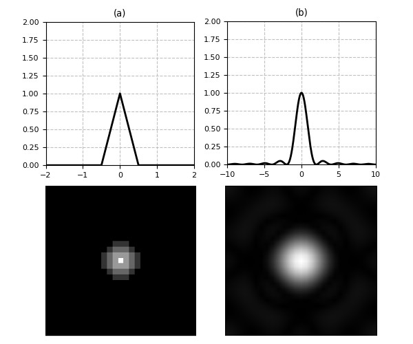
The frequency response of the Gaussian filter is much better behaved than all the others discussed so far. In fact, the Fourier transform of a Gaussian is another Gaussian that monotonically and asymptotically decreases to zero. This means that there are no ripples in the stop-band and, therefore, no frequency leakages so that local details are better preserved, as can be seen in Fig.11 (in reality, due to the discretization process the curve is not perfectly flat and there are still some minor oscillations, but their effect is much less evident compared to box filters).
Also, and more interestingly, since the frequency response is still a Gaussian it has a spread parameter \(\sigma_F\), and it can be shown that such parameter is tied to the filter’s \(\sigma\) by the following relation
$$ \sigma^2_F = \frac{1}{\sigma^2} \tag{6}$$
that is by increasing the spread in the filter, the range of allowed frequencies becomes narrower and, vice versa, decreasing the filter’s spread will expand the range of allowed frequencies. This is a very important parameter at disposal of the designer that can choose the best trade-off between the strength of the smoothing effect and the amount of high frequency components (that is of details) to be preserved.
Another very interesting property is its separability into the product of two functions in lower dimensions. In 2D, in fact, the Gaussian (4) can be written as the product of two 1-dimensional Gaussians, as follows
$$ \begin{align} h(i,j;\sigma) & = k e^{-\frac{i^2+j^2}{2 \sigma^2}} \\ & = k \left[ e^{-\frac{i^2}{2 \sigma^2}} \cdot e^{-\frac{j^2}{2 \sigma^2}} \right] \\ & = k [h(i;\sigma) \cdot h(j;\sigma)] \end{align} \tag{7}$$
so the kernel can be decomposed as follows
$$ h = h_i \cdot h_j \tag{8}$$
where \(h_i\) and \(h_j\) are two orthogonal vectors. These two 1-dimensional kernels can then be convolved with the image separately in cascade, with the consequence of a reduction in computational complexity.
The Gaussian filter is widely used for the regularization of images affected by “grainy” noise, which is typically a Gaussian type of noise and occurs naturally in many physical processes. To see its response to a noisy image of this kind we use the same corrupted image used for the box filters and process it with the kernel (5). The results are shown in Fig.12
Notice how despite the use of bigger kernels many details of the original image are still visible in the smoothed images. This is because the Gaussian filter is able to reduce the noise while retaining more details compared to uniform smoothing filters. However, this example just demonstrates the differences using the specific kernels in (5). Remember that the Gaussian filter is parametric and different results can be obtained by finding the value of \(\sigma\) that gives the best trade-off between noise reduction and preservation of details.
Even though both Gaussian and box filters are not capable of suppressing impulsive type of noise without heavily deteriorating the details, box filters are generally more effective than Gaussian filters in this case (at parity of kernel size) because of their stronger blurring effect, unless the standard deviation of the Gaussian is set to a value larger than the size of the kernel, in which case it degenerates into a box filter. Fig.13 shows the response of the Gaussian filter to an image affected by “salt & pepper” noise.
The reason of the poor performance for this use case is the same as for the box filters: impulsive noise introduces pixels with extremely high (or low) intensity that are usually very unrepresentative of the local features and the linear process of averaging can’t totally suppress the heavy impact they have in the computation without compromising the details. The best method to eliminate this type of noise would be that of excluding these pixels from the computation altogether, which is what some non-linear filters do, as we’ll see in a next article.