We have seen how smoothing filters can be used to remove details from images by suppressing low frequency components with the effect of making them blurred. Sharpening filters do just the opposite. They emphasize regions with high spatial frequency in order to highlight details. The basic idea underlying all sharpening filters is that of boosting sudden variations of intensity, that is transitions from dark to bright areas (or vice versa), as those are indication of important visual cues (the “details”), while ignoring regions of slowly changing or constant intensity, usually representing featureless areas.
Suppose that we want to enhance an image, because it’s been deteriorated by some process, such as blurring, or simply because we want to improve its quality to make it visually more appealing or prepare it for further processing. Then we can think of restoring the lost details (or enhancing the existing ones) using a simple additive operation
$$ g_e = g + g_d \tag{9}$$
where \(g_e\) is the enhanced image resulting from adding elements \(g_d\) to the original (possibly degraded) image \(g\). To better understand how this is achieved we need to figure out what those “elements” added to the image actually are.
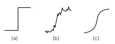
The way humans visually perceive and recognize objects is based on variations of luminosity in the 2D space, which form important visual cues used by the brain to process images, such as lines, corners, points and blobs. All these transitions can be represented as shown in Fig.10 and are commonly referred to as edges in the literature. They are of particular importance because usually associated with parts of an image that are visually meaningful.
In Fig.11 is a real-world example where 3 segments of pixels have been extracted from 3 different regions of an image. These segments contain significant changes of intensity connected to visual cues indicating the presence of objects in the scene, such as a boat (a), the sails ropes and mast (b) and the portholes (c).
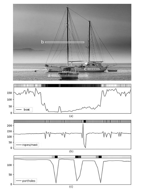
The graphs in Fig.11 show the intensity profiles of the 3 segments and it can be noted that whenever an object appears in the scene there is a transition taking place indicating the presence of an edge. Due to noise and textures, the edges in real-world images are usually not as smooth as the model in Fig.10(c), but that’s a very good approximation, especially if the image has been subject to blurring.
Also, depending on the nature of the objects, the edges may manifest in different forms, generally as step-like or pulse-like transitions. The step-like edge represents a typical transition found in boundaries between homogeneous objects (Fig.11(a)), while the pulse-like is typically associated with isolated points or lines (Fig.11(b,c). However, impulsive transitions can be seen as the combination of two specular step transitions, so we can usually consider this as a general model for all edges.
With these concepts in mind we can now elaborate more on equation (9) and find out what those “elements” \(g_d\) added to the image for enhancement are. If we take the derivative of the image then in the presence of an edge we get a strong response that indicates some important visual cue. Once these elements have been found, they can be used to enhance the image by performing a simple linear combination. The details of the image can be represented by a high-pass filtered version of it, and the sharpening done using the following equation
$$ g_e(x) = g(x) + k \cdot D[g(x)] \tag{10}$$
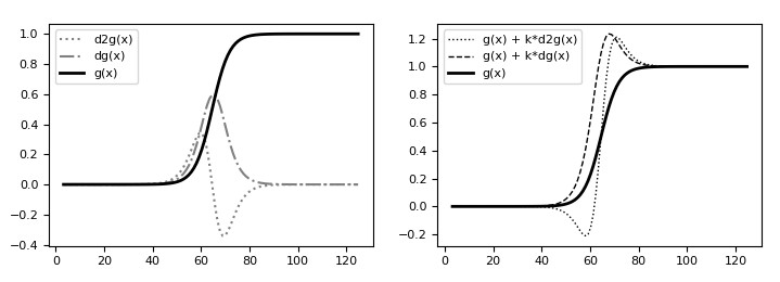
where \(D[g(x)]\) is a differential function of the image, that is any mathematical operator using its derivatives, and \(k\) a constant parameter controlling the strength of the sharpening. Fig.12 shows an example of this method in one dimension using the first and second derivative of the signal.
Due to the properties of differentiation, the sharpening operation basically enhances high frequency components while leaving untouched those that are constant or slowly changing, thus effectively acting like a high-emphasis filter. This technique is known as differential filtering and is widely used in image processing and, particularly, in computer vision due to the edges being the main feature by which humans recognize shapes and objects.
In order to be effectively used in (10), \(D[g(x)]\) should satisfy the following properties
- Linearity, as we want to implement it as a linear filter
- Discriminative between areas of highly varying intensity, where the details lie, and homogeneous “featurless” areas
- Accuracy, as we want the details being reconstructed with good precision
- Noise-resistance, for reliability
Since differential operators produce strong responses to high frequency components of the signal and are insensitive to low frequency or constant components, any filter using such operators can basically be considered as a high-pass filter. We will now discuss various types of differential (high-pass) filters used to perform edge detection and will analyze their performances in the sharpening of images. As a side note, and to avoid confusion in the use of terms, “edge detection” here refers to finding the intensity transitions in images in order to enhance the details and not to extract “contours” (or “boundaries”) of objects, which usually require further analysis and have different purposes.
Gradient filters
These filters are based on the gradient operator and are also called first order differential filters. The gradient provides information about how a multivariate function changes in its domain, so it’s a suitable tool to implement the sharpening operation according to equation (10). It satisfies properties 1, 2 and 3, as it’s a linear operator, responds to highly changing signals while being insensitive to slowly changing or constant ones, and can detect edges with good accuracy. It does not satisfy property 4 (as with all differential filters) but some variants can mitigate this issue.
In practice, it is not possible to mathematically compute the analytical expression of the gradient for digital images, as it’s only defined for continuous functions. But it enjoys some properties, specifically linearity, locality and translation invariance, that allow for its definition as a linear filter, and thus applied using a discrete convolution operation
$$ \nabla g(x,y) = \begin{bmatrix} \frac{\partial g(x,y)}{\partial x} \\ \frac{\partial g(x,y)}{\partial y} \end{bmatrix} = \begin{bmatrix} (h_{\nabla x} * g)(x,y) \\ (h_{\nabla y} * g)(x,y) \end{bmatrix} \tag{11}$$
where \(h_{\nabla x}\) and \(h_{\nabla x}\) are two suitable kernels defining the derivatives of the image along the x and y directions. There are several definitions of \(h_{\nabla x}\) and \(h_{\nabla x}\) in the literature used to approximate the gradient. Here we’ll examine the most commonly used in the field of image processing highlighting their pros and cons.
Simple gradient filter
The simplest approximation of the gradient can be achieved by using the forward (or backward) finite difference to calculate the derivatives. Using the forward difference, for example, we can estimate the derivative of a function with sufficient accuracy using the following equation
$$ \frac{df(x)}{dx} \approx f(x+1) – f(x) \tag{12}$$
so the gradient of an image can be written as follows
$$ \nabla g(x,y) = \begin{bmatrix} \frac{\partial g(x,y)}{\partial x} \\ \frac{\partial g(x,y)}{\partial y} \end{bmatrix} \approx \begin{bmatrix} g(x+1,y) – g(x,y) \\ g(x,y+1) – g(x,y) \end{bmatrix} \tag{13}$$
from which we can write the convolution kernels \(h_{\nabla x}\) and \(h_{\nabla y}\)
$$ h_{\nabla x} = \begin{bmatrix} -1 & 1 \\ 0 & 0 \end{bmatrix} \hspace{10pt} h_{\nabla y} = \begin{bmatrix} -1 & 0 \\ 1 & 0 \end{bmatrix} \tag{14}$$
The gradient of the image is generally a scalar field computed using the gradient’s magnitude by convolving the image with both kernels and combining the resulting derivative images according to the following equation
$$ \left\Vert \nabla g \right\Vert = \sqrt{(h_{\nabla x} * g)^2 + (h_{\nabla y} * g)^2} \tag{15}$$
or an approximation using the following more computationally efficient equation
$$ \left\Vert \nabla g \right\Vert \approx \left\Vert h_{\nabla x} * g \right\Vert + \left\Vert h_{\nabla y} * g \right\Vert \tag{16}$$
the orientation of the gradient can also be estimated as follows
$$ \phi(\nabla g) = tan^{-1} \left( \dfrac{h_{\nabla y} * g}{h_{\nabla x} * g} \right) \tag{17}$$
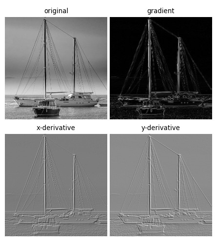
An example of the results produced by this filter is shown in Fig.13.

We can then use the resulting gradient to sharpen the original (possibly degraded) image according to (10) using the following equation
$$ g_e = g + k \cdot \left\Vert \nabla g \right\Vert \tag{18}$$
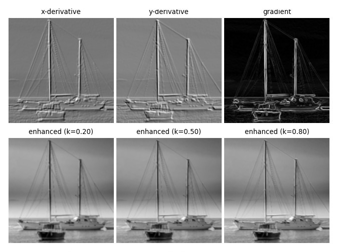
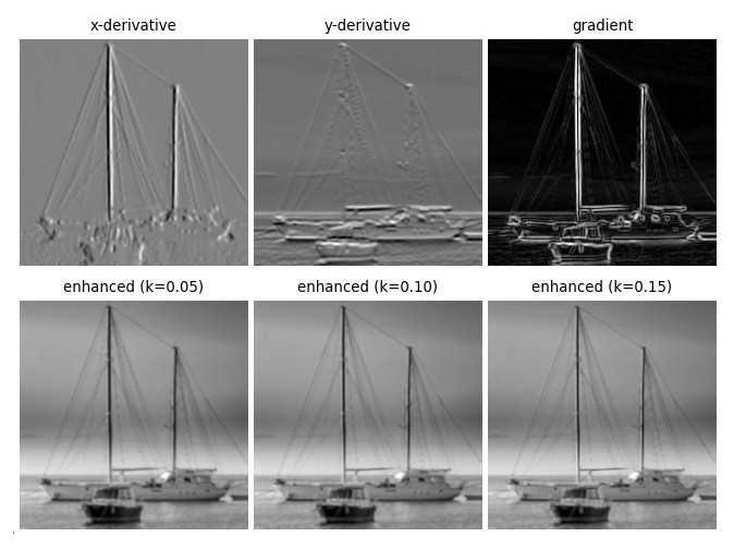
where \(\left\Vert \nabla g \right\Vert\) represents the details of the image that need to be emphasized and \(k\) is a parameter that controls the strength of the sharpening effect. Fig.14 below shows the application of a simple gradient filter to sharpen a blurred image using different values of \(k\) (note that the image derivatives have been normalized in the range [0, 255] for display purposes, but keep in mind they have negative values too)
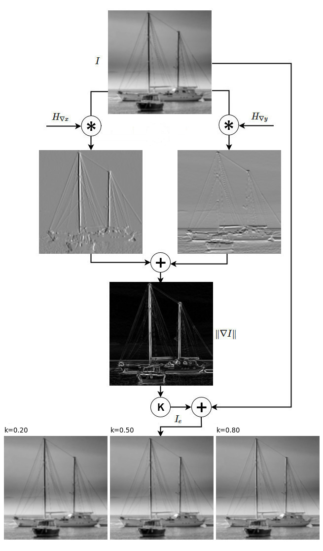
The image at the top is the original blurred using a Gaussian filter. The 3 images at the bottom are the result of applying the sharpening filter (18) using 3 different values of \(k\). It can be noticed how the filter has somewhat reconstructed the details that were blurred away by the smoothing operation, even though the sharpening effect is not great. The resulting image, in fact, does not have very clear features due to the way this type of filter emphasizes the edges. We’ll see this in more details later on when we will discuss higher order differential filters.
The value of k is crucial as it regulates the amount of details to be restored in the image, thus determining its sharpness. This value depends on the strength of the high-pass filter’s response and also on the application, so generally there is no “optimal” value. As a rule of thumb it should be set to a number smaller than one. However, and more importantly, if its value is too high it may cause excessive emphasis on the transitions resulting in distortions that manifest as “halos” around the edges.
Another drawback of gradient filters is that they are anisotropic, that is their response is strongly dependent on the orientation of the image (they’re not rotation-invariant). This means that edges are not detected equally well in all directions, and if the image has a different orientation the response will change, leading to the same edges being detected and sharpened with different quality. Below is a Python implementation of the sharpening filter (18)
import numpy as np
import cv2 as cv
import matplotlib.pyplot as plt

ipath="/path/to/image"

g = cv.imread(ipath, cv.IMREAD_GRAYSCALE).astype(np.float32)
g /= 255
gs = cv.GaussianBlur(g, (5, 5), 1)

hx = np.array([[0, 0, 0],
               [0,-1, 1],
               [0, 0, 0]])

hy = np.array([[0, 0, 0],
               [0,-1, 0],
               [0, 1, 0]])

dgx = cv.filter2D(gs, -1, hx)
dgy = cv.filter2D(gs, -1, hy)
dg = np.sqrt(dgx**2 + dgy**2)

ke = [0.2, 0.5, 0.8]
ge = [(gs, "blurred")]

for k in ke:
    img = np.clip(gs + k * dg, 0, 1)
    gp = (img, "enhanced (k=%1.2f)" % k)
    ge.append(gp)

implot([
    ge, [(dg, "gradient")]
])
Roberts filter
This filter is a variation of the simple gradient filter wherein the derivatives are computed on a 45-degree rotated coordinate system so that its maximum response is on edges diagonal to the considered point. The gradient of this filter is given by
$$ \nabla g(x,y) = \begin{bmatrix} \frac{\partial g(x,y)}{\partial x} \\ \frac{\partial g(x,y)}{\partial y} \end{bmatrix} \approx \begin{bmatrix} g(x,y) – g(x+1,y+1) \\ g(x+1,y) – g(x,y+1) \end{bmatrix} \tag{19}$$
and the kernels \(h_{\nabla x}\) and \(h_{\nabla y}\) are defined as follows
$$ h_{\nabla x} = \begin{bmatrix} 1 & 0 \\ 0 & -1 \end{bmatrix} \hspace{10pt} h_{\nabla y} = \begin{bmatrix} 0 & 1 \\ -1 & 0 \end{bmatrix} \tag{20}$$
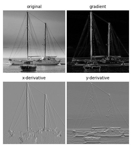
the image gradient and the gradient’s orientation are computed as in the simple filter using (16) and (17). Note that since this filter uses a crossed pattern on a 2×2 kernel the resulting gradient is actually an approximation of the gradient at \((x+\frac{1}{2}, y+\frac{1}{2})\). The results produced by this filter are shown in Fig.15
They are similar to those of the simple gradient filter as they’re practically based on the same principles. However, it can be observed that the Roberts filter has detected more edges in the derivative images. This is because the orientation of the image is better suited for this filter compared to the simple gradient. If we rotate the image by 45 degrees we would get pretty much the same results as the simple gradient’s, demonstrating their poor isotropic properties.
Figure 15.2 below shows the results of the application of Roberts filter to sharpen the same image used for the simple gradient filter.
Roberts filter’s main advantage lies in its low computational cost due to the small size of the kernel and the use of simple addition and subtraction operations on integers. However, this point of strength is much less valuable today with more powerful computers allowing the use of more sophisticated filters at a comparable processing speed. Despite this, it may still be useful in resource-constrained devices, such as embedded systems and microchips.
Sobel filter
Another gradient-based filter with a different (and better) implementation compared to other filters in the same class is the Sobel filter, which is defined as follows
$$ \begin{align} \nabla g(x,y) &= \begin{bmatrix} \frac{\partial g(x,y)}{\partial x} \\ \frac{\partial g(x,y)}{\partial y} \end{bmatrix} \\[2ex] & \approx \begin{bmatrix} \begin{matrix} g(x+1,y+1)-g(x-1,y-1) \\ +2(g(x+1,y)-g(x-1,y)) \\ +g(x+1,y-1)-g(x-1,y-1) \end{matrix} \\[2ex] \begin{matrix} g(x+1,y-1)-g(x+1,y+1) \\ +2(g(x,y-1)-g(x,y+1)) \\ +g(x-1,y-1)-g(x-1,y+1) \end{matrix} \end{bmatrix} \end{align} \tag{21}$$
from which we can define the matrices \(h_{\nabla x}\) and \(h_{\nabla y}\)
$$ h_{\nabla x} = \begin{bmatrix} -1 & 0 & 1 \\ -2 & 0 & 2 \\ -1 & 0 & 1 \end{bmatrix} \hspace{10pt} h_{\nabla y} = \begin{bmatrix} 1 & 2 & 1 \\ 0 & 0 & 0 \\ -1 & -2 & -1 \end{bmatrix} \tag{22}$$
The image gradient and its orientations can, again, be computed using (16) and (17). As can be noted, this approximation of the gradient uses the central difference instead of the forward difference, which provides for a more accurate estimation of the derivatives. Notably, these derivatives are taken at and around the central pixel along the x and y directions, with the central one having a bigger weight. The idea of this method is that of getting an estimate of the gradient at each point as a weighted average of the gradients that can be computed in a 3×3 neighborhood, resulting in a better approximation and conferring better isotropic properties compared to the other gradient filters. The results produced by this filter can be seen in Fig.16

From the gradient image we can see that the Sobel filter is able to capture more polished details compared to the other filters. If we look at the derivative images we can see that they are smoother, thus producing a smoother gradient. Also, the filter has a stronger response yielding thicker and bolder edges. All this is because of the larger kernel and the way it is designed. In fact, the filter is actually separable, that is it can be decomposed into the product of 2 orthogonal vectors \(uv^T\) as follows
$$ h_{\nabla x} = \begin{bmatrix} 1 \\ 2 \\ 1 \end{bmatrix} \cdot \begin{bmatrix} -1 & 0 & 1 \end{bmatrix} \hspace{10pt} h_{\nabla y} = \begin{bmatrix} -1 \\ 0 \\ 1 \end{bmatrix} \cdot \begin{bmatrix} 1 & 2 & 1 \end{bmatrix} \tag{23}$$
With this decomposition the Sobel filter can be seen as the combination of a smoothing triangular filter in one direction and a derivative filter in the orthogonal direction, which combined give a smoothed gradient. The separation also reduces the computational complexity of the convolution and allows for more efficient implementations.
Fig.16.2 shows the application of the Sobel filter to sharpen the same image used in the previous examples.

The enhanced images appear to be slightly better compared to those produced using the other gradient filters (but this is subjective), and it required a smaller sharpening factor due to its stronger response.
Prewitt filter
The Prewitt filter is basically a variant of the Sobel filter where the derivatives have all the same weights
$$ h_{\nabla x} = \begin{bmatrix} -1 & 0 & 1 \\ -1 & 0 & 1 \\ -1 & 0 & 1 \end{bmatrix} \hspace{10pt} h_{\nabla y} = \begin{bmatrix} 1 & 1 & 1 \\ 0 & 0 & 0 \\ -1 & -1 & -1 \end{bmatrix} \tag{24}$$
Like Sobel’s, it’s separable into the product of 2 vectors, as follows
$$ h_{\nabla x} = \begin{bmatrix} 1 \\ 1 \\ 1 \end{bmatrix} \cdot \begin{bmatrix} -1 & 0 & 1 \end{bmatrix} \hspace{10pt} h_{\nabla y} = \begin{bmatrix} -1 \\ 0 \\ 1 \end{bmatrix} \cdot \begin{bmatrix} 1 & 1 & 1 \end{bmatrix} \tag{25}$$
which is a combination of average filtering in one direction and derivative filter in the orthogonal direction. It gives similar results as the Sobel filter, as can be seen in Fig.16.3
The results of the sharpening using this filter are shown in Fig.16.4
One advantage over the Sobel filter is that it only performs additions and subtractions of the elements and there are no other operations involved. There is another benefit in the use of this filter on noisy images, as we’ll see in the next section.
Effects of noise
The major drawback of gradient filters is their sensitivity to noise. This should not come as a surprise though since they act like high-pass filters and are therefore not able to suppress noisy components that generally lie on the high end of the spectrum. Fig.16.5 shows how the gradient filters discussed in so far respond to an image corrupted with additive Gaussian noise
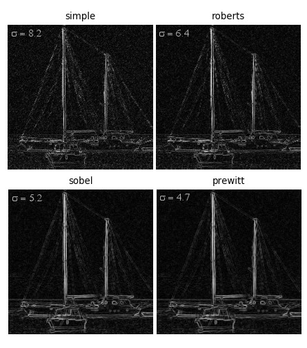
The simple gradient filter has the highest sensitivity to noise since it shows the worst response, as also indicated by the highest local standard deviation. The Roberts filter has a better response, probably due to the fact that the gradients are computed at an interpolated point producing some smoothing effect on the noise. The Sobel and Prewitt filters have the best response because of their inherent smoothing properties, which filter out a consistent part of the noise. In particular, the Prewitt filter performs the best, likely due to the fact that it uses an average filter in one direction, which has a higher blurring effect compared to the triangular filter used by Sobel.
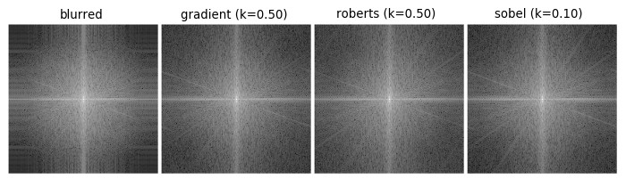
Effectiveness of sharpening
Even though a qualitative analysis shows that first order high-pass filters do not yield quality results for image enhancement, a quantitative analysis will demonstrate that the processed images are indeed sharper and details have been restored. This can be seen in Fig.16.6, which depicts the frequency responses of the original image and sharpened images. It is evident that high frequency components, where the details lie, have been somehow brought back. The problem is that the quality is not visually satisfactory from a perceptual point of view.
The reason first order derivative filters are not very effective in the sharpening of images is due to their limited dynamics that make them unable to enhance an edge so that its transition produces a strong acutance (perceived sharpness), similar to the ideal step-like model shown in Fig.10. We will see in the next section how differential filters of higher order can accomplish this task and give much better results.
Laplacian filters
The sharpening filters based on the computation of the gradient belong to the class of first order derivative (or differential) filters. Another class of differential filters that satisfies properties 1, 2 and 3 (but again not 4 out of the box) is the so called Laplacian, which is based on the computation of the second derivatives of the signal. For this reason, they are also called second order differential filters. The second derivative of a discrete signal can be approximated using the central difference, which is calculated like so
$$ \begin{aligned} \frac{d^2 f(x)}{dx^2} & \approx f(x+1) – f(x) – (f(x) – f(x-1)) \\ & = f(x+1) – 2f(x) + f(x-1) \end{aligned} \tag{26}$$
Using this approximation, the Laplacian of an image can be defined as follows
$$ \begin{aligned} \nabla^2 g(x,y) & = \frac{\partial^2 g(x,y)}{\partial x^2} + \frac{\partial^2 g(x,y)}{\partial y^2} \\[2ex] & \approx \begin{matrix} g(x+1,y) + g(x-1,y) + g(x,y+1) + \\ g(x,y-1) – 4g(x,y) \end{matrix} \end{aligned} \tag{27}$$
which, again, can be expressed as a linear filter and applied by convolution with the image \(g\)
$$ \nabla^2 g(x,y) = (h_{\nabla} * g)(x,y) \tag{28}$$
where \(h_{\nabla}\) is defined by the following matrix
$$ h_{\nabla} = \begin{bmatrix} 0 & 1 & 0 \\ 1 & -4 & 1 \\ 0 & 1 & 0 \end{bmatrix} \tag{29}$$
The kernel (29) can easily be extended by calculating the second derivatives on the other 4 directions to get the following variant
$$ h_{\nabla} = \begin{bmatrix} 1 & 1 & 1 \\ 1 & -8 & 1 \\ 1 & 1 & 1 \end{bmatrix} \tag{30}$$
Other variants of \(h_{\nabla}\) are possible, depending on how the derivatives are approximated. A common one is obtained by inverting the verses of the derivatives resulting in a sign change in the elements of the kernel, which provide equivalent results but are sometimes more convenient in the calculations.
$$ h_{\nabla} = \begin{bmatrix} 0 & -1 & 0 \\ -1 & 4 & -1 \\ 0 & -1 & 0 \end{bmatrix} \hspace{10pt} h_{\nabla} = \begin{bmatrix} -1 & -1 & -1 \\ -1 & 8 & -1 \\ -1 & -1 & -1 \end{bmatrix} \tag{31}$$
There are a few interesting properties about the Laplacian filter that make it a better choice over gradient filters in many applications. First of all, it can immediately be noted that it is an isotropic filter, meaning it is rotation-invariant (i.e. not depending on the orientation of the image) and responds to intensity changes equally well in all directions.
Another peculiarity is its better accuracy in detecting edges compared to gradient filters due to the use of second order derivatives, and this has important consequences in the enhancement of images using equation (10). We have already seen the second derivative of the edge model (Fig.12, left) and the difference of performing the sharpening using both the first and second derivative (Fig.12, right). This difference will be more clear looking at the 2D examples shown in Fig.17.
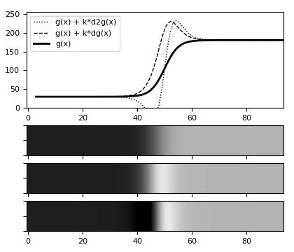
The plot at the top in Fig.17 depicts the transition of a blurred edge (thick line) along with its sharpened versions produced by equation (10) using the first derivative (dashed line) and the second derivative (dotted line). The three images underneath represent the same edges in the 2D space, specifically the blurred edge (top), the enhanced version using the gradient filter (middle), and the enhanced version using the Laplacian filter (bottom).
It can be seen how the Laplacian sharpens the edge much better than the gradient filter. This is because the first derivative produces a pulse-like response (a Gaussian) at the centre of the edge that enhances the signal along the whole transition. So, when used in equation (10), the edge is emphasized on the bright side and also on the darker side causing the bright details to be smeared across, as can be seen in Fig.17.
On the other hand, the second derivative has a more articulated response that produces two opposite pulses that emphasize the edge on the bright side and de-emphasize it on the darker side, giving it a sharper profile. This also approximates very well a neural process that allows humans to detect edges, called the Mach bands effect. As a consequence, when used with equation (10) the results are visually much better (note that the second derivative must be inverted for the filter to work properly).
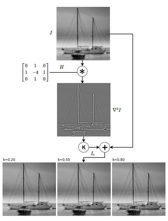
Enhancing an image using the Laplacian filter only requires one convolution. Once the differential (Laplacian) image has been computed, the sharpening of the image can be performed according to (10) using the following equation
$$ g_e = g \pm k \cdot \nabla^2 g \tag{32}$$
where the sign depends on whether the used kernel has a positive or negative central element (must be the same as the central element’s). Fig.18 shows an example of the sharpening using the Laplacian filter at varying values of the parameter \(k\).
The whole sharpening process can be performed in one single operation by rewriting equation (32) considering the distributive property of convolution, as follows
$$ \begin{align} g_e & = (\pm h_1 * g) + k(h_{\nabla} * g) \\ & = (\pm h_1 + kh_{\nabla}) * g \\ & = \pm (h_e * g) \end{align} \tag{33}$$
where \(h_1\) is the identity kernel (a matrix with the central element set to 1 and all others to 0) and \(h_e\) the sharpening kernel that results from adding the identity and Laplacian kernels. Again, the sign must be chosen according to the Laplacian’s central element sign. For example, if (29) was used then the sharpening kernel would be
$$ h_e = -h_1 + kh_{\nabla}= \begin{bmatrix} 0 & 0 & 0 \\ 0 & -1 & 0 \\ 0 & 0 & 0 \end{bmatrix} + k \begin{bmatrix} 0 & 1 & 0 \\ 1 & -4 & 1 \\ 0 & 1 & 0 \end{bmatrix} \tag{34}$$
Note that if the Laplacian’s central element is negative then the original image will be inverted, so the resulting sharpened image \(g_e\) must be inverted as well. In this case it’s probably better to use the variants with positive central element defined as follows (assuming k=1)
$$ h_e = \begin{bmatrix} 0 & -1 & 0 \\ -1 & 5 & -1 \\ 0 & -1 & 0 \end{bmatrix} \hspace{10pt} h_e = \begin{bmatrix} -1 & -1 & -1 \\ -1 & 9 & -1 \\ -1 & -1 & -1 \end{bmatrix} \tag{35}$$
One major drawback of this filter is its high sensitiveness to noise. In fact, since it is more effective at sharpening transitions than gradient filters it will also be more responsive to those caused by noise, as it operates linearly. For this reason in practical applications the Laplacian is usually used in conjunction with a smoothing filter and the process of filtering consists of two steps: low-pass filtering for noise reduction and differential filtering for edge detection. The low-pass filter is typically a Gaussian one and the whole process can be expressed using only one convolution operation
$$ \nabla^2 \bigl( h_{\sigma}*g \bigr)(x,y) = \bigl( \nabla^2 h_{\sigma} * g \bigr)(x,y) \tag{36}$$
where the Laplacian is applied to the image smoothed with the Gaussian filter \(h_{\sigma}\), defined by the following function
$$ h_{\sigma}(x,y) = \frac{1}{2 \pi \sigma^2} \cdot e^{-(x^2+y^2)/2\sigma^2} \tag{37}$$
and the kernel \(\nabla^2 h_{\sigma}\) is called the Laplacian of Gaussian (LoG), which is derived by applying the Laplacian operator to (37)
$$ \begin{align} \nabla^{2} h_{\sigma}(x,y) = h_{LoG} & = \frac{\partial^{2}h_{\sigma}(x,y)}{\partial x^2} + \frac{\partial^2 h_{\sigma}(x,y)}{\partial y^2} \\[2ex] & = \frac{x^2+y^2-2\sigma^2}{2 \pi \sigma^6} e^{-(x^2+y^2)/2\sigma^2} \end{align} \tag{38}$$
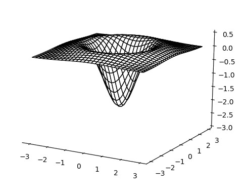
If we plot (38) the resulting function is very similar to a simple Laplacian filter controlled by the parameter \(\sigma\), as shown in Fig.19. For small values of \(\sigma\), in fact, the LoG in a discrete space degenerates into a simple Laplacian, which means that filtering with a too small \(\sigma\) has no smoothing effect.
A LoG kernel can be derived from the 2D LoG function (38) by approximation with discrete values using an appropriate \(\sigma\) (the size of the kernel \(m\) should be odd and satisfy \(m \geq 5\sigma\)). In order for the filter to have differential properties the sum of the elements in the kernel must be zero. An example of LoG kernel that approximates the function for \(\sigma=1.2\) is given below
$$ h_{LOG} = \begin{bmatrix} 0 & 0 & 1 & 1 & 1 & 0 & 0 \\ 0 & 1 & 1 & 2 & 1 & 1 & 0 \\ 1 & 2 & -2 & -5 & -2 & 2 & 1 \\ 1 & 3 & -5 & -10 & -5 & 3 & 1 \\ 1 & 2 & -2 & -5 & -2 & 2 & 1 \\ 0 & 1 & 1 & 2 & 1 & 1 & 0 \\ 0 & 0 & 1 & 1 & 1 & 0 & 0 \end{bmatrix} \tag{39}$$
Consider now an image corrupted with random noise and processed with both a simple Laplacian and a LoG. The results are shown in Fig.20.
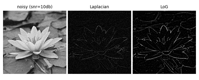
The image in Fig.20 has been corrupted with additive Gaussian noise and filtered with the simple Laplacian (29) and the LoG (39). It can be seen how the Laplacian filter is extremely sensitive to noise, leading to all the noisy transitions being detected with equal magnitude as the real edges, many of which have been wiped out. The LoG filter, on the other hand, reduces a lot of the noise and finds the edges by clearly separating them from the noisy background. Even though there is still a residual amount of noise it can easily be filtered out with further processing, for example by thresholding the image. A side effect is that the edges will be subject to blurring too and are thicker than those produced by the Laplacian.
Unsharp mask filter
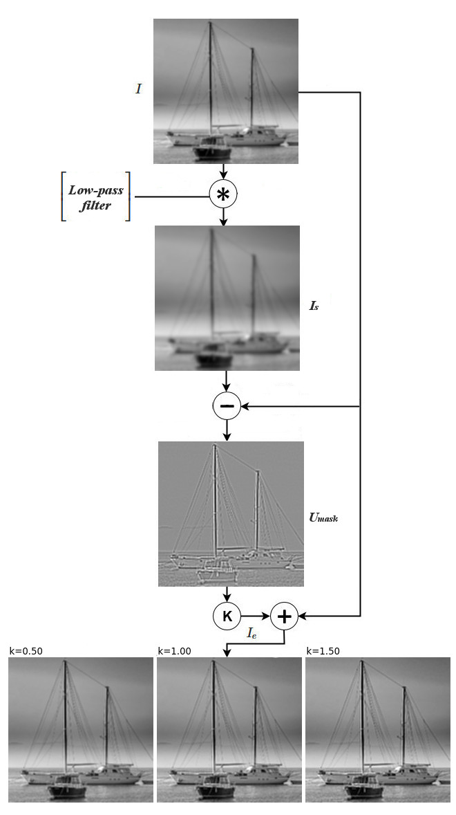
The last filter that will be discussed is called Unsharp Mask filter. The idea behind it is very simple: given an image, if we subtract a smoothed (low-pass filtered) version from it then the resulting image will contain only the high frequency components, that is all the edges. We can then use this image to combine it with the original in order to enhance the details. In formal terms the Unsharp Mask filter is given by the following equation
$$ g_e = g + k (g – g_s) \tag{40}$$
which is basically another form of equation (10). The term \((g – g_s)\) represents the “unsharp mask”, that is the edges obtained by subtracting from the original image a smoothed version \(g_s\). This latter operation essentially implements a high-pass filter. Fig.21 shows the Unsharp Mask filter along with the results on the test image used in the previous examples
It can be proven that the Unsharp Mask filter is equivalent to the Laplacian sharpening filter (32). In fact, rewriting the definition of Laplacian given in (27) for reasons of brevity
$$ \nabla^2 g(x,y) = N(x,y) – 4g(x,y) \tag{41}$$
where \(N(x,y)\) represents the image evaluated at all neighboring points of \((x,y)\), then the sharpening filter (32) can be written as follows
$$ \begin{align} g_e(x,y) & = g(x,y) + k \cdot \nabla^2 g(x,y) \\ & = g(x,y) + k \cdot \Bigl(N(x,y) – 4g(x,y) – g(x,y) + g(x,y)\Bigr) \\ & = g(x,y) + k \cdot -\frac{1}{5} \Bigl(g(x,y) – \frac{1}{5} \left[g(x,y) + N(x,y)\right]\Bigr) \\ & = g(x,y) + k \cdot -\frac{1}{5} \Bigl(g(x,y) – g_s(x,y)\Bigr) \end{align} \tag{42}$$
that is, applying the Laplacian can be seen (net of a constant factor) as subtracting from each point of the original image an average of all the points in the kernel, which is indeed a smoothed version of the original image. Following is a Python implementation of the Unsharp filter
import numpy as np
import cv2 as cv
import matplotlib.pyplot as plt

ipath="/path/to/image"

g = cv.imread(ipath, cv.IMREAD_GRAYSCALE).astype(np.float32)
g /= 255
g = cv.blur(g, (3, 3))
um = g - cv.GaussianBlur(g, (5, 5), 1)

ke=[0.5, 1, 1.5]
ge=[(g, "blurred")]

for k in ke:
    img = np.clip(g + k * um, 0, 1)
    gp = (img, "enhanced (k=%1.2f)"%k)
    ge.append(gp)

implot([
    ge,
    [(um, "Unsharp Mask")]
])
Conclusion
Linear sharpening filters are a simple but effective tool to improve the details in images, whether for mere visual reasons or to optimize further processing. At their core are the high-pass filters, in their different flavors. We have seen that second order high-pass filters are the best choice for this task, and are those that are typically used in practice. However, high-pass filters are not only limited to uses for image enhancement. Another important application, and probably the most common in image processing, is for contours extraction, which is an essential task in computer vision in order to detect the boundaries of objects for segmentation.